Travel-time curve calculation for the Spherical Earth (PREM Model)

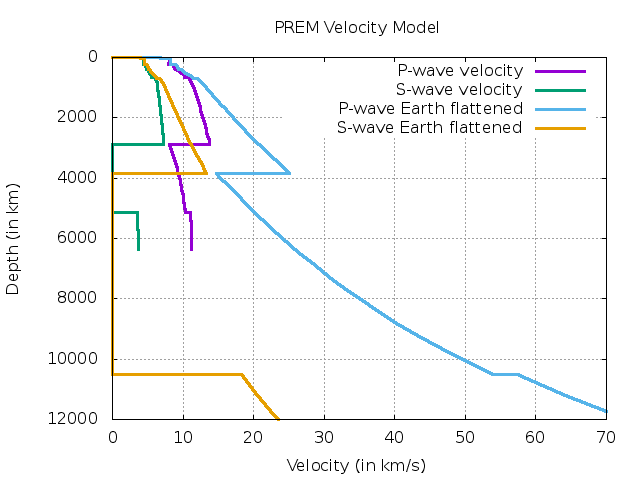
I have used the Preliminary Reference Earth Model of Dziewonski and Anderson (1981) to calculate the travel time curve. This model is very robust in the sense that it is designed to fit a wide variety of data including free-oscillation, surface wave dispersion observations, , travel time data for a number of body wave phases etc. To download the model, click here.

The travel time curve is the plot of first arrival time of a ray from source to receiver vs the epicentral distance (surface to surface) traveled. The sum of the time taken by the ray in each layer from the source to the receiver gives the total travel time. The ray path depends on the ray-parameter (which is constant for a laterally homogeneous, flat layers). Ray with different ray-parameter will propagate along different paths for a given earth model. For a normal velocity model (velocity increases with depth), smaller ray parameters will turn deeper in Earth and hence travel farther. The ray-parameter (p) varies along the travel time curve and is give by its slope at an instant.

I have taken two approach to calculate the travel time; first by modeling the earth using laterally homogeneous layers, and second by modeling using the velocity gradient. For details see Chapter 4, Shearer, 2009.

In the first case, I stack all the layers and the distance traveled by the ray is calculated by summing the travel time in each layer until the ray turns (which is decided by comparing slowness and ray-parameter value). When the slowness (reciprocal of velocity) of the layer is equal to the ray-parameter, the ray turns in that medium and then start traveling towards the surface. There is an inherent uncertainty associated with this method depending on the thickness and large number of the layer.

In different approach, we can parametrize the velocity model at a number of discrete points in depth and evaluate the distance and travel time by assuming an appropriate interpolation function between the model points. Here, for my calculation, I have considered the linear velocity gradient in the layer.

We have used the Earth-flattening transformation to calculate the travel-time for the spherical Earth. The curvature of the travel time curve in a spherical Earth can be simulated in a flat Earth model if a special velocity gradient is introduced in the half-space (Mu¨ller, 1971; Shearer, 2009).

The Earth-Flattening Transformation applied to the PREM Model

Fortran Program for layered earth model:

program comp_travel_time
 !Calculates the travel time data for a layered, flat earth for given layer thicknesses and velocities
 implicit none
 real, parameter :: pi = 2*asin(1.0), a=6371
 integer, parameter:: np=401
 real(kind=16), allocatable, dimension(:) :: delztmp, delz, slow, vel, eta, slowS, velS, etaS, utop, ubot, ustop, usbot
 real(kind=16) :: xx0, xx, tt0, tt, delz0, rr, pinit,pend, dp, xx0S, xxS, tt0S, ttS
 integer:: i,j,numl, nlyr
 real(kind=16), dimension(1:np) :: p
 character*11 :: file1 !name of the model file
 CHARACTER(len=32) :: arg1 !number of layers as argument
 CALL get_command_argument(1, arg1)
 read(arg1, '(I2)') numl
 allocate(delztmp(1:numl), delz(1:numl), slow(1:numl), vel(1:numl), eta(1:numl), &
 slowS(1:numl), velS(1:numl), etaS(1:numl),utop(1:numl), ubot(1:numl), ustop(1:numl), usbot(1:numl))

file1='ps_prem.dat' !model file name
 i=1
 open(1,file=file1, status='old')
 do while (i .le. numl)
 read(1,*) delztmp(i), vel(i), velS(i) !layer thickness and vel from file
 call read_data(delztmp(i), vel(i), velS(i))
 i=i+1
 end do
 close(1)
 i=1
 j=1
 do while(i .le. numl) !For flat Earth, calculate the layer thickness, and average velocity
 delz(j)=delztmp(i+1) - delztmp(i)
 utop(j)=vel(i)
 ustop(j)=velS(i)
 ubot(j)=vel(i+1)
 usbot(j)=velS(i+1)
 vel(j)=(utop(j)+ubot(j))/2
 velS(j)=(ustop(j)+usbot(j))/2
 !write(*,'(i2,3f12.2)') j, delz(j), vel(i), vel(i+1)
 nlyr=j
 i=i+1
 j=j+1
 end do
 nlyr=nlyr-1 !total number of layers

pinit=0.0017 !lower bound of ray parameter range
 pend=0.1128 !upper bound of ray parameter range
 dp=(pend-pinit)/np
 !write(*,'(a,1x,a,1x,a,1x,a)') "p in s/km","X(p) in km","X(p) in degrees","Time in mins"
 do j=1,np
 p(j)=pinit + (j-1)*dp !ray paramter increasing by dp 
 xx0=0
 xx0S=0
 tt0=0
 tt0S=0
 !P-wave calculation
 do i=1,nlyr
 slow(i)=1/vel(i) !in s/km
 if (slow(i) .gt. p(j) .and. slow(i) .le. 100000) then
 call travel_time_calc(xx0,tt0,slow(i),p(j),delz(i),eta(i),xx,tt)
 end if
 !S- wave calculation
 slowS(i)=1/velS(i)
 if (slowS(i) .gt. p(j) .and. slowS(i) .le. 100000) then
 call travel_time_calc(xx0S,tt0S,slowS(i),p(j),delz(i),etaS(i),xxS,ttS)
 end if
 end do
 
 open(2, file='p_travel_time.dat')
 write(2,'(f12.4,1X,f12.2,1X,f12.3,1X,f12.2)') p(j), xx, xx*(360/(2*pi*a)), tt/60
 !write(*,'(f12.4,1X,f12.2,1X,f12.3,1X,f12.2)') p(j), xx, xx*(360/(2*pi*a)), tt/60

open(3, file='s_travel_time.dat')
 write(3,'(f12.4,1X,f12.2,1X,f12.3,1X,f12.2)') p(j), xxS, xxS*(360/(2*pi*a)), ttS/60
 !write(*,'(f12.4,1X,f12.2,1X,f12.3,1X,f12.2)') p(j), xxS, xxS*(360/(2*pi*a)), ttS/60
 end do
 
 deallocate(delztmp, delz, slow, vel, eta, slowS, velS, etaS) 
end program comp_travel_time


!!SUBROUTINES


!reading the p, and s wave velocity, and depth from the model and convert it from spherical to flat earth
subroutine read_data(delztmp, vel, velS)
 real, parameter :: pi = 2*asin(1.0), a=6371
 real(kind=16):: delztmp, vel, velS
 real(kind=16) :: rr
 rr=a-delztmp !distance from the center of earth
 delztmp=-a*log(rr/a) !earth flattening transformation
 vel=(a/rr)*vel !earth flattening transformation for velocity
 velS=(a/rr)*velS !earth flattening transformation for shear velocity
 return
end

!Calculation of surface to surface distance of source and receiver and the travel time of ray
subroutine travel_time_calc(xx0,tt0,slow,p,delz,eta,xx,tt)
 real(kind=16) :: eta,slow,p,xx,xx0,delz,tt,tt0
 eta=sqrt(slow**2 - p**2)
 xx=xx0+(2*p*delz*(1/eta))
 tt=tt0+(2*slow**2*delz*(1/eta))
 xx0=xx
 tt0=tt
end

 

To compile and run this program:

datafile=ps_prem.dat
rm -f $datafile *.exe
awk 'NR>2{print $1,$3,$4}' PREM_MODELorg.model > $datafile
if [ ! -f "$datafile" ]; then #When the velocity model is not provided
cat >$datafile<<eof
3 4 3
6 6 5
9 8 7
eof
fi

numl=`wc -l $datafile | awk '{print $1}'`
prog="comp_travel_time.f95"
 
exect=`echo $prog | cut -d"." -f1` #execuatable

gfortran $prog -o ${exect}.exe 
if [ -f "${exect}.exe" ]; then
./${exect}.exe $numl #argument is the number of layers

For the velocity gradient model, the fortran program is below. For this case, I have made use of the LAYERXT subroutine based on Chris Chapman’s WKBJ Program.

program comp_travel_time_vel_grad
 !Calculates the travel time data for a layered, flat earth for given layer thicknesses and velocities
 implicit none
 real, parameter :: pi = 2*asin(1.0), a=6371
 integer, parameter:: np=501
 real(kind=16), allocatable, dimension(:) :: delztmp, delz, vel, velS, utop, ubot, ustop, usbot
 real(kind=16) :: rr, pinit,pend, dp, delz0, xx, tt, xxS, ttS, xx0,tt0, xx0S, tt0S
 integer:: i,j,numl, nlyr,irtr, irtrS
 real(kind=16), dimension(1:np) :: p
 character*12 :: file1 !name of the model file
 CHARACTER(len=32) :: arg1 !number of layers as argument
 CALL get_command_argument(1, arg1)
 read(arg1, '(I2)') numl
 allocate(delztmp(1:numl), delz(1:numl), vel(1:numl), &
 utop(1:numl), ubot(1:numl), ustop(1:numl), usbot(1:numl), velS(1:numl))


 file1='ps_prem.dat' !model file name
 i=1
 open(1,file=file1, status='old')
 open(5,file='flat_earth.dat')
 do while (i .le. numl)
 read(1,*) delztmp(i), vel(i), velS(i) !layer thickness and vel from file
 rr=a-delztmp(i) !distance from the center of earth
 delztmp(i)=-a*log(rr/a) !earth flattening transformation
 vel(i)=(a/rr)*vel(i) !earth flattening transformation for velocity
 velS(i)=(a/rr)*velS(i) !earth flattening transformation for shear velocity
 write(5,'(i2,3f12.2)') i, delztmp(i), vel(i), velS(i)
 i=i+1
 end do
 close(1)
 i=1
 j=1
 do while(i .le. numl) !For flat Earth
 delz(j)=delztmp(i+1) - delztmp(i)
 utop(j)=1/vel(i)
 ustop(j)=1/velS(i)
 ubot(j)=1/vel(i+1)
 usbot(j)=1/velS(i+1)
 !write(*,'(i2,3f12.2)') j, delz(j), vel(i), vel(i+1)
 nlyr=j
 i=i+1
 j=j+1
 end do
 nlyr=nlyr-1 !because of singularity at earth's center
 write(*,*) "size_delz", nlyr
 pinit=0.0017 !lower bound of ray parameter range
 pend=0.1128 !upper bound of ray parameter range
 dp=(pend-pinit)/(np-1)
 do j=1,np
 p(j)=pinit + (j-1)*dp !ray paramter increasing by dp
 xx0=0
 xx0S=0
 tt0=0
 tt0S=0
 irtr=100
 irtrS=100
 do i=1,nlyr
 if (irtr .ne. 2) then
 call layerxt(p(j),delz(i),utop(i),ubot(i),xx,tt,irtr)
 xx=xx0+xx
 tt=tt0+tt
 xx0=xx
 tt0=tt
 else
 exit
 end if
 end do
 open(2, file='p_travel_time.dat')
 write(2,'(f12.4,1X,f12.2,1X,f12.3,1X,f12.2)') p(j), 2*xx, 2*xx*(360/(2*pi*a)), 2*tt/60
 !write(*,'(f12.4,1X,f12.2,1X,f12.3,1X,f12.2)') p(j), xx, xx*(360/(2*pi*a)), tt/60
 do i=1,nlyr
 if (ustop(i) .le. 100000 .and. usbot(i) .le. 100000) then
 if (irtrS .ne. 2) then
 call layerxt(p(j),delz(i),ustop(i),usbot(i),xxS,ttS,irtrS)
 xxS=xx0S+xxS
 ttS=tt0S+ttS
 xx0S=xxS
 tt0S=ttS
 else
 exit
 end if
 end if
 end do
 open(3, file='s_travel_time.dat')
 write(3,'(f12.4,1X,f12.2,1X,f12.3,1X,f12.2)') p(j), 2*xxS, 2*xxS*(360/(2*pi*a)), 2*ttS/60
 !write(*,'(f12.4,1X,f12.2,1X,f12.3,1X,f12.2)') p(j), xxS, xxS*(360/(2*pi*a)), ttS/60
 end do
 write(*,'(a,1x,a,1x,a,1x,a)') "p in s/km","X(p) in km","X(p) in degrees","Time in mins"
 deallocate(delztmp, delz, vel, &
 utop, ubot, ustop, usbot, velS) 
end program comp_travel_time_vel_grad

!!SUBROUTINES


! LAYERXT calculates dx and dt for a ray in a layer with a linear 
! velocity gradient. This is a highly modified version of a 
! subroutine in Chris Chapman's WKBJ program.
!
! Inputs: p = horizontal slowness
! h = layer thickness
! utop = slowness at top of layer
! ubot = slowness at bottom of layer
! Returns: dx = range offset
! dt = travel time
! irtr = return code
! = -1, zero thickness layer
! = 0, ray turned above layer
! = 1, ray passed through layer
! = 2, ray turned in layer, 1 leg counted in dx,dt
!
subroutine LAYERXT(p,h,utop,ubot,dx,dt,irtr)
 implicit none
 real(kind=16) :: p, h, utop, ubot,dx, dt, u1,u2,v1,v2,b,eta1,x1,tau1, &
 dtau,eta2, x2,tau2
 integer :: irtr
 if (p.ge.utop) then !ray turned above layer
 dx=0.
 dt=0.
 irtr=0
 return 
 else if (h.eq.0.) then !zero thickness layer
 dx=0.
 dt=0.
 irtr=-1
 return 
 end if

u1=utop
 u2=ubot
 v1=1./u1
 v2=1./u2
 b=(v2-v1)/h !slope of velocity gradient

eta1=sqrt(u1**2-p**2)

if (b.eq.0.) then !constant velocity layer
 dx=h*p/eta1
 dt=h*u1**2/eta1
 irtr=1
 return
 end if

x1=eta1/(u1*b*p)
 tau1=(log((u1+eta1)/p)-eta1/u1)/b

if (p.ge.ubot) then !ray turned within layer,
 dx=x1 !no contribution to integral
 dtau=tau1 !from bottom point
 dt=dtau+p*dx
 irtr=2
 return
 end if

irtr=1

eta2=sqrt(u2**2-p**2)
 x2=eta2/(u2*b*p)
 tau2=(log((u2+eta2)/p)-eta2/u2)/b

dx=x1-x2
 dtau=tau1-tau2

dt=dtau+p*dx

return
end

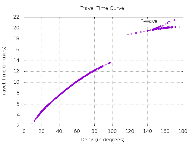
In the travel-time curve, we can notice the general increase of travel time with delta. We can notice the large shadow zone around 100 degrees. This is because of the P wave transition from the solid mantle to the liquid core; which leads to sharp decrease in velocity. This is the low-velocity zone, where the rays are bent downward. So, no rays originating at the surface can turn within the LVZ. If the seismic rays originate inside the LVZ, it can never get trapped within the zone. If the seismic attenuation is lower in the LVZ layer, then the wave originated in it can propagate a long distance (Optical fiber cables work on the same principle).

X(p) curve for P-wave

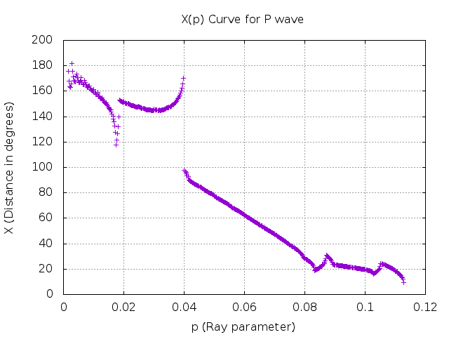
In general, the epicentral distance increases as the p decreases. When the X increases with decreasing p, the branch of the travel time curve is prograde otherwise called retrograde. The retrograde branch can be observed occasionally because of the rapid velocity transition in the Earth. The point of change from prograde to retrograde is called caustics; where X value does not change with p. At this point, the energy is focussed since the rays with different p values (or take off angles) arrive at same range(X). We can also notice in the above X(p) curve that there is sharp change in X around 0.02 and 0.04. Around 0.02, the slope is positive, which could be because of the rapid velocity transition in Earth. Since, for lower p value, the ray travels deeper; this could be the inner core boundary (ICB). This is because at ICB, the P-wave velocity increases drastically.  At point 0.04, the slope is large negative; which could be the core-mantle boundary.

• Utpal Kumar (IES, Academia Sinica)

Reading Complex Text Data (MATLAB)

Text data which is in one format all through the file is easier to read. But when the text data has numeric entries, string entries (different data formats), then it becomes little complicated to read and write. Sometimes, the data is also not arranged in regular rows and columns form which makes them even more tougher to read.

Here we address such problems.

Reading complex text data

Reading Data

clear; close all; clc;

filename='stn_data.txt'; %giving the file name to be opened

fileID = fopen(filename); %defining the identifier for file

format='%s %f %f'; %format of the text file

data=textscan(fileID,format);

fclose(fileID); %close the file

stnName=data{1};    %reading the first column

data1=data{2};  %reading the second column

data2=data{3};  %reading the third column

Writing Data:

clear; close all; clc;

%% Writing Data into the text file

%defining a number of strings

stnName={'ABC','DEF','GHI','JKL','MNO','PQR','STU','VWX','YZA'}; 

%defining variable data1 with values between 0-10

data1=10*rand(1,length(stnName));

%defining variable data1 with values between 0-100

data2=100*rand(1,length(stnName));

fileid=fopen('stn_data.txt','w'); %opening a file in writing mode

for i=1:length(stnName)

    fprintf(fileid,'%s %.3f %.3f\n',stnName{i},data1(i),data2(i)); %writing data into the file iteratively

end

fclose(fileid); % closing the file

MATLAB Scripts:

Reading data

Writing data

Using a Function (MATLAB)

If we need to run the same algorithms or formula for computations again and again, then instead of writing the same stuffs in our script file many times, we can simply write a function. This makes our script look simpler and faster to run.

Writing a function in MATLAB

Examples:

Calculating mean and standard deviation

Calculating distance from origin

Calculates distance (in km) between two coordinate points on the Earth’s surface

Writing and Reading Simple Text Data (MATLAB)

Working with text data is convenient as we can share our data with other systems without giving them the trouble to install a particular software to read our data.

Let’s see how we can read and write a text data using MATLAB.

Reading text data in MATLAB

Reading text Data

%% Reading the data in text file

fileID = fopen('nums.txt','r'); %opeing the file in reading mode

p=fscanf(fileID,'%s %s',2); %reads the header

formatSpec = '%d %f'; %defining the format of the data

sizeA = [2 Inf]; %defining the size of the data

A = fscanf(fileID,formatSpec,sizeA); %reading the data using fscanf function

fclose(fileID); %closing the file

A' %displaying the data

Writing Text Data

clear; close all; clc;

%% Defining the variables

x = 1:10;

y = [x;10*rand(1,10)]; %randomly generated 2nd column

z=['x-values' '  ' 'random-values']; %writing the header

%% Writing the data in text file

fileID = fopen('nums.txt','w'); %opens a text file in writing mode

fprintf(fileID,'%s %s %s\n',z);

fprintf(fileID,'\n');

fprintf(fileID,' %d         %4.4f\n',y); %write the data y in the file. 

%The first column is written in digit format and second column in floating point format.

fclose(fileID); %close the file

MATLAB Scripts:

Reading text data

Writing text data

Reading Data from Microsoft Excel (MATLAB)

The MATLAB is very easy to use language. This is one of the main reason why it is getting popular day by day.

Here, we show how we can read data from the Microsoft excel into the MATLAB. Once we can read the data into the MATLAB, we can do other computations and operations quite easily.

Reading Excel Data in Matlab

Sample data file (global_temp.xlsx)

Matlab script to read global_temp.xlsx

Saving data in Mat or text format for easier and faster use in later programs

Aliasing and Nyquist Condition

Let us consider a simple sinusoidal signal

x(t) = 5sin(10t + 3)

This is a signal with an amplitude of 5, the angular frequency of 10 and phase of 3. The Nyquist condition demands that the angular frequency, mod(𝜔) ≤ pi/delta t.

For the above figure 1, we took 𝜔 to be 10 and pi/delta t is 99.5, so the Nyquist condition satisfies and we do not see the aliasing. Here the sampling rate, Δ𝑡 is 0.0316.

Let us see what happens when we take the pi/delta t to be less than 𝜔.

In this case, we took the sampling rate, Δ𝑡 to be 0.3307. Here the pi/delta t is 9.5000 which is less than 𝜔. Hence the Nyquist condition is not satisfied and there is a clear aliasing. The sinusoidal signal does not appear to be sinusoidal.

Figures

Singular Value Decomposition

The inversion of a matrix is a very important part of data analysis. The quality of inverse solution depends on how well we can invert the matrix.

d=Gm where “d” is the N dimensional column vector consisting the data, “m” is the M dimensional column vector consisting the model parameters which we seek to invert for, “G” is the NxM dimensional kernel matrix to map the model vectors into the data matrix.

=>m = Ad, where A is the inverse of the matrix G.

There are several matrix decomposition techniques. These techniques are not only useful for the inverse problems, but also for applications like principal decomposition that are widely used in seismic attribute studies.

When a matrix is pre-multiplied to a vector, the resultant vector can be regarded as a linear transformed version of the original vector. Therefore the multiplication of matrices is a linear transformation. Any matrix can generally be decomposed into transformations of some other matrices.

The decomposition of a general rectangular matrix requires the use of singular value decomposition or SVD (Lanczos, 1961). The SVD decomposes any rectangular matrix A of m rows and n columns into a multiplication of three matrices of useful properties:

A = U L V’

Here, L is the m x n rectangular diagonal matrix containing p singular values (or principal values) of the matrix A.

U and V are the two square unitary matrices. The number of non-trivial singular values, p is called the trace or rank of the matrix.

We try to solve for the an example of

A = (10  2; -10 2)

Example 1