Calculating Auxiliary Fault Plane Solutions given the main fault (Fortran)

We have calculated the auxiliary fault plane solution using the input of main fault solution in perl. Here, we do the same in Fortran. And we will also plot to solution to visualize the results.

Fortran Code to get the auxiliary fault plane solutions:

program auxiliary_fault_plane
! Program to calculate the strike, dip and rake of the auxiliary fault plane solutions
! given the strike, dip and rake of the fault plane.
! Authors: Utpal Kumar, Li Zhao
        implicit none
        real (kind=8):: ph1,del1,lb1,ph2,del2,lb2,sinlb2,coslb2,sinph1_ph2,cosph1_ph2,ph1_ph2,phI,delI,lbI
    real, parameter :: pi = 2*asin(1.0)
    integer :: n,lbsgn

        print *, 'Enter strike, dip and rake respectively of the fault plane (in degrees) (e.g., 40,50,60):'
        read *, ph1,del1,lb1
        !ph1=40
        !del1=80
        !lb1=200
        phI=ph1
    delI=del1
    lbI=lb1
        !Converting the strike, dip and rake in radians
        ph1=ph1*pi/180  !strike
        del1=del1*pi/180        !dip    
        lb1=lb1*pi/180          !rake   
        
        !Adaptation to include the negative values of rake
        lbsgn=1
        if (lb1 < 0) then
                lbsgn=-1
        end if
        
        
        ! Calculation of Strike, sip and rake of the auxiliary fault plane
        del2=acos(sin(lb1)*sin(del1))   !dip of auxialiary fault plane
        sinlb2=cos(del1)/sin(del2)
        coslb2=-(sin(del1)*cos(lb1)/sin(del2))
        lb2=acos(coslb2)        !rake of auxilairy fault plane
        sinph1_ph2=cos(lb1)/sin(del2)
        cosph1_ph2=-1/(tan(del1)*tan(del2))
        ph1_ph2=acos(cosph1_ph2)

        !Checking for the quadrant of the strike angle
        if (sinph1_ph2 >= 0 .and. cosph1_ph2 >=0) then
        ph1_ph2=ph1_ph2
        else if (sinph1_ph2 > 0 .and. cosph1_ph2 < 0) then
        ph1_ph2=ph1_ph2
        else if (sinph1_ph2 < 0 .and. cosph1_ph2 < 0) then
        ph1_ph2=-ph1_ph2
        else if (sinph1_ph2 < 0 .and. cosph1_ph2 > 0) then
        ph1_ph2=-ph1_ph2
        end if
        
        ph2=ph1-ph1_ph2         !strike of auxialiary fault plane
        
        ! For dip > 90 degrees and less than 180 degrees
        if (del2 > pi/2 .and. del2 < pi) then
        ph2= pi + ph2
        del2= pi - del2
        lb2= 2*pi - lb2
        end if
        
        if (lbsgn < 0) then
                lb2 = -(2*pi - lb2)
        end if
        
        !Adaptation to give the strike value in the range of 0 to 360 degrees
        if (ph2 > 2*pi) then
                ph2 = ph2 - 2*pi
        end if
        
        101 format("The strike of the auxiliary plane is: ",f9.4, " degrees")
        102 format("The dip of the auxiliary plane is: ",f9.4, " degrees")
        103 format("The rake of the auxiliary plane is: ",f9.4, " degrees")
        print 101, ph2*180/pi
        print 102,  del2*180/pi
        print 103, lb2*180/pi
    open(unit=10,file='plt.dat')
    10 format("25  25   0 ",  f8.2, f8.2, f8.2, f8.2, f8.2, f8.2," MainFault: ",f7.2,"/",f7.2,"/",f7.2, &    !continuation of line
        " AuxFault: ",f7.2,"/",f7.2,"/",f7.2)
        write(10,10) phI,delI,lbI,ph2*180/pi, del2*180/pi, lb2*180/pi, phI,delI,lbI,ph2*180/pi, del2*180/pi, lb2*180/pi !writing in the file
end program auxiliary_fault_plane

Then we save this in the file called “auxiliary_fault_plane.f”. This script basically aim for calculation of the fault plane solution. For visualizing the results, we can execute the program and plot the results using the psmeca command of GMT.

The bash script for compiling and executing the above program and then plotting it is following:

#!/bin/bash
gfortran -ffree-form auxiliary_fault_plane.f -o auxiliary_fault_plane
./auxiliary_fault_plane
psbasemap -Bwsne -R0/50/0/50 -Jm1.0 -Xc -Yc -P -K >output.ps
echo "24.6 30 20 0 2 MC Focal Mechanism Plot"| pstext -Jm -R -K -O -P -N >>output.ps
psmeca plt.dat -Jm -R -Sa0.40/14/-0.2i -Gbrown -Fa0.2c/cd -Egray -P -O -N -L -V >>output.ps

gs output.ps
ps2pdf output.ps

The P axis is plotted using circle and T axis using the diamond symbol (-Fa0.2c/cd).

-Utpal Kumar (IES, Academia Sinica)

Calling SAC(Seismic Analysis Code) (in Perl)

For seismologists, using a SAC for sac data manipulation is essential (though there are few alternatives). Here, we see how can we call SAC from a perl script:

#!/usr/bin/perl
open(SAC, "| sac ") or die "Error opening sac\n";
print SAC qq[
echo on
*fg seismogram    #sample seismic signal in SAC's memory
fg sine 2 npts 2000 delta 0.01
*fg impulse npts 100 delta 0.01
bandpass bessel corner 0.1 0.3 npole 4
ppk
fft
plotsp am
save sine_fft.pdf
];
print SAC "quit\n";
close(SAC);

Example script to call SAC functions in perl

Some utilities to deal with sac data format

In seismology, we usually have to deal with the sac data format (binary data format). This data format can be dealt easily and efficiently with the SAC software provided by IRIS. But if we want to use this data in other software for instance MATLAB, then we may need to convert the data in alphanumeric format or to install additional functions.

Here, we show how can we deal with the sac data file format.

1. If you have sac installed on your system, then you can make use of the sac’s “convert” command to convert the data from alphanumeric format to sac format, back and forth.
2. There are several other functions and libraries available online to deal with the sac data file format directly in MATLAB. For example, Mike Thorne’s Software, Frederik J. Simons Repository
3. Here we give some useful utilities:

prem is a simple program to return the PREM velocities and density for an input depth. Using this you don’t need to check manually what is the PREM velocity at a particular depths.

This can be compiled using the following steps:

g95 -c getprem_mod.f90

g95 prem.f90 -o prem ./getprem_mod.o

mkdir -p ~/bin

mv prem ~/bin

sachead returns the value of specified sac header. So, you don’t need to read the data with sac to get its header information. If you have sac already installed in your computer then you don’t need this utility as there is a utility “saclst” which does the same job.

usage: >> sachead sacfile headervariable

To compile this utility,

g95 -c mod_sac_io.f90

g95 sachead.f90 -o sachead mod_sac_io.o

mkdir -p ~/bin

mv sachead ~/bin

sac2xy converts the sac file from binary to alphanumeric format

usage: >> sac2xy sacfile outputfile

For compilation,

g95 -c mod_sac_io.f90

g95 sac2xy.f90 -o sac2xy  mod_sac_io.o

mkdir -p ~/bin

mv sac2xy ~/bin

To add these programs into the path of your system,

open “~/.bashrc” file using your favourite text editor

add the following line to it

export PATH=$PATH:~/bin

close the .bashrc file and restart your terminal window or run “.  ~/.bashrc” command

Or directly from the terminal,

type

echo “export PATH=$PATH:~/bin” >> ~/.bashrc

Mac users can add the following lines to the file ~/.bash_profile

C-shell users can edit the ~/.cshrc file.

echo “setenv PATH $PATH\:/~/bin” >> ~/.cshrc

We list some MATLAB functions which can be used directly to import sac data in MATLAB:

1. load_sac : To read header and sac data
2. rmean : To remove mean from the read sac data
3. rtrend : To remove linear trend from the data
4. cos_taper : Applies a 10% cosine taper
5. bp_bu_co : Bandpass filter using butterworth filter implementation

Statistical Analysis in MATLAB

 

Histogram plot

Monte-Carlo simulation for testing hypothesis

Probability Density plot

Doing statistical analysis in MATLAB is lot easier than other computer languages. Here, we can make use of the intrinsic “plot” to visualize the statistics of the data.

Below are some programs for commonly used statistical analysis:

1. Calculating mean, standard deviation, median etc of the data and visualizing the data using the histograms. Here, we do the example for a random normal and non-normal data. : Statistics 1
2. Histogram Plotting
3. Hypothesis Testing
4. Monte-Carlo Simulations and calculating the p-value
5. Probability distribution plots of the data
6. t-test statistics

Data file for test run of some of the above programs: temp_month.mat 

Simple Numerical Tests on Tomography

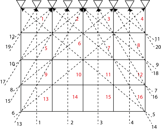
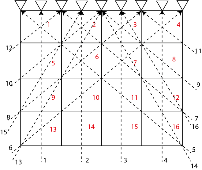
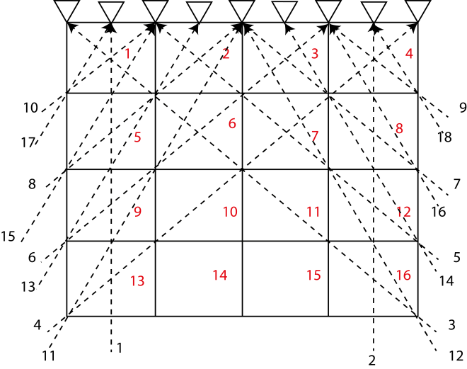
Numerical Tests on tomography

Tomography, which is derived from the Greek word “tomos” that is “slice”, denotes

forming an image of an object from measurements made from slices or rays through

it. In other words, forming the structure of an object based on a collection of slices

through it.

In principle, it is usually an inverse problem where we have the data, we formulate the

geometry of the ray paths and invert for the model parameters that defines the

structure.

d = Gm

where, d is the vector containing the data, m is the vector containing the model

parameters and G is the kernel which maps the data into the model and vice-versa.

If there are N number of data and M number of model parameters then the size of the

matrix G is M×N.

The first step of this problem is to formulate a theoretical relationship between the

data and model spaces and the underlying physics. Once, this theoretical relationship

is established or the matrix G is formulated, we can address the above problem in two

ways – a forward problem or an inverse problem.

The forward problem can be taken as a trial and error process or as an exhaustive

search through the model space for the best set of model parameters which can reduce

the misfit between the observed and the predicted data. For this case, we guess the

model based on the simple real world geology and then determine the data based on

the theoretical relationship between data and models. In contrast, in the inverse

problem we invert for the model parameters using the data and considering the

theoretical relationship between the data and model parameters. Then we interpret for

the real world geology.

The solution of the linear tomographic inverse problem depends on the relationship

between Nand M. If N < M, then we have more number of model parameters or

variables to obtained and lesser number of data or equations to solve. In this case, the

equation d = Gm does not provide enough information to determine uniquely all the

model parameters and thus the problem is called underdetermined. We usually need

extra constraints to solve this kind of problem, for example we take the a priori

constraint that the solution to this problem is simple. If N = M, then there is ideally

enough information to determine the model parameters. But in real world, data is

usually inaccurate and inconsistent to invert for the best model parameters in this

case. If N > M, there is too much information contained in the equation d = Gm for

it to possess an exact solution. This case is called the overdetermined.

Overdetermined Problem

Equal – Determined Problem

Mixed-Determined Problem

Understanding Seismograms

Seismograms are basic information about earthquakes, chemical and nuclear explosions, mining induced earthquakes, rock bursts and other events generating seismic waves.

Seismograms reflect the combined influence of the seismic source, the propagation paths, the frequency response of the recording instrument and the ambient noise at the recording site.

u(t) = s(t)*g(t)*i(t)*n(t).         “*” means convolution.

where, u is the seismic record, s is the source effect, g is the propagation effect, i is the instrument effect and n is the noise.

So, by understanding seismogram we can understand the seismic source, earth structure, and the noise in the medium.

This is our short attempt to understand the seismograms.

Understanding Seismograms 1

For understanding the seismogram, there are two main things we should notice- record duration and the dispersion. Due to different nature of the propagation velocity of the seismic waves and the different propagation paths taken by them to the station, travel time differences between the main group usually grows with distance. Since the body wave groups do not disperses, so their individual duration remains more or less constant, only the time difference between them changes with distance.

Figure 1: Event-Station Distribution map for the event in Mindanao, Phillipines Island (2005-02-05, Mw-7). The source is 540 km deep.

Figure 2

Figure 3

Figure 4

The epicentral distance for QIZ, BJT and DGAR is ~ 19, 35, 52 degrees respectively. For the station BJT (Figure 3), the epicentral distance is 35.2 degrees and for the station DGAR (Figure 4), the epicentral distance is 52.4 degrees. The P-S arrival times for the station BJT is nearly 300 sec and for the station DGAR, the P-S arrival time is nearly 400 sec. For the station QIZ, it is only around 200 sec. So, with the increase in epicentral distance, the difference in individual phase arrival increases. Also for the station DGAR, the P arrival is later than the BJT.

The time difference between main body wave onsets is:

Distance (degrees) less than	Time-difference in body wave onsets (P-S) in sec
10	180
60 (Fig 1,2,3)	960
100	1800
180	2700

Figure 5 : Travel-Time curve for depth 540 km

For the deep events, we do not see the first arrival as P wave (Figure 6) for short distances (D

Figure 6

Figure 6, is the seismogram at 2 degrees epicentral distance from the deep source. Here, we can notice that the first arrival is not P but the core reflected phase PcP. It is also cevident from the travel time curve(Figure 5).

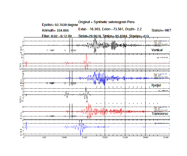
Figure 7: Event-Station Distribution Map of Near Coast of Peru (2001-06-23, Mw-8.3). The source is at 2 km depth.

When the source is near the surface then we observe the surface waves as well in the seismogram.The surface waves from earthquakes at intermediate (> 70 km) or great depth (> 300 km) may have amplitudes smaller than those of body waves or may not even be detected on seismic records.

In contrast to the body waves, the velocity of surface waves is frequency dependent and hence it is dispersed. The duration of Love and Rayleigh waves increases with distance. As for station NNA (Figure 8), the duration of the first group of Rayleigh wave is about 230 seconds and for station HKT (Figure 9), the duration is around 600 seconds.

We can also notice that for shallower earthquake event, P-wave is the first arrival for stations less than 10 degrees of the source (Figure 10).

Figure 8

In Figure 8, we can notice that for surface waves, the largers periods arrive first than the lowers periods. This is the general case for normal layering. The larger periods sample the higher depths and since the velocity for higher depths is larger so it arrives before the shorter period waves.

Figure 9

In figure 9, for the surface waves, we can observe the wave groups or the beating effect (analogous to acoustics). This is because of the interference of the two or more harmonic waves with closer frequencies or periods.

Figure 10: Travel time curve for depth 2.2km

For certain distance ranges, the travel time curves for different types of seismic phases are close to each other or can even overlap (Figure 5,11).

(a)

(b)

 Figure 11: S, SKS and ScS are very close to each other.

The amplitude of P-wave depends not only on the epicentral distance but on the site effect (underground geology and crustal heterogeneity), azimuth etc.

The most obvious indication on a seismogram that a large earthquake has a deep focus is the small amplitude of the surface waves with respect to the body-wave amplitudes and the P and S waveforms often have impulsive onsets.

A more precise determination of the depth h of a seismic source, however, requires either the availability of a seismic network with at least one station being very near to the source, e.g., at an epicentral distance D < h (because only in the near range the travel time t(D, h) of the direct P wave varies strongly with source depth h), or the identification of seismic depthphases on the seismic record.

At distant seismograph stations, the depth phases pP or sP follow the direct P wave by a time interval that changes only slowly with distance but rapidly with depth.