Simple 1D velocity model inversion from P arrival time

Refer to Chapter 5, Introduction to Seismology, Shearer 2009.

Problem:

From the P-wave travel time data below (note that the reduction velocity of 8km/s), inverse for the 1D velocity model using T(X) curve fitting (fit the T(X) curve with lines, then invert for the ray parameter p and delay time τ(p), then solve for the velocity and depth).

 

Fig 1. P-wave travel time from a seismic experiment.

 

Solution:

We construct the T(X) plot from the data: y = T  – X/8 => T = y + X/8 and then divide the T(X) curve into fitting lines (Fig. 2).

Fig 2. T(X) plot with lines fitting to data points.

The ray parameter and delay is calculated for each line by using:

p = dT/dX

τ = T – pX

These parameters p and τ are slope and intercept of a line, respectively.

The τ(p) can be written as:

as in the matrix form of:

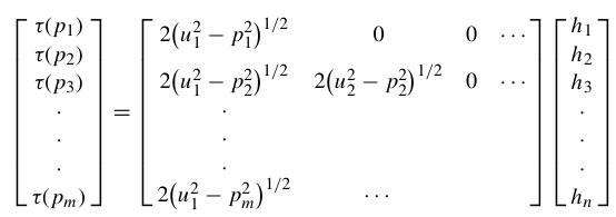
or, in short,

We can invert for the thickness of each layer using least square inversion:

If we assume ray slowness u(i) = p(i) for each line, we can solve the h and v for the 1D velocity model.

Here is the result of the inversion:

The sharp increase in Vp from ~6.6 km/s to 7.7 km/s at ~ 30km depth suggest for the Moho discontinuity.

The codes for the problem is written in python and can be downloaded: source code, τ inversion code, data points.

Nguyen Cong Nghia, IESAS