Complex Moving Waves

In the previous case, we have seen how can we model a simple wave travelling with one frequency. In nature, usually we encounter waves as an ensemble of many frequencies.

Here, let us try to add more frequencies in the previous scenario:

MATLAB code

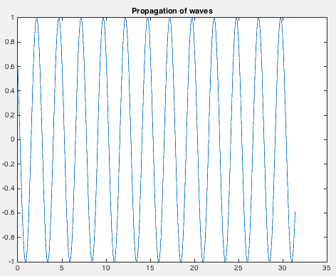
clear; close all; clc

fs=1000;    %sampling frequency

t=0:1/fs:0.5-1/fs;%time

f=[1 2 3];  %frequency1

a=[1 2 3];  %amplitude

c=2; %wave speed

T=1./f;  %time period

w=2*pi*f;   %angular frequency

lb=c*T; %wavelength

k=(2*pi)./lb; %wavenumber

x=0:pi/200:(2.5*pi)-pi/200;

figure('Position',[440 378 800 500])

for i=1:length(t)/2

%     y=a*sin(k*x-w*t(i));    %waveform

    y=a(1)*sin((k(1)*x)-(w(1)*t(i))+0.3)+a(2)*sin((k(2)*x)-(w(2)*t(i))+0.4)+a(3)*sin((k(3)*x)-(w(3)*t(i))+0.5);

    plot(x,y,'--*')

    title('Propagation of waves')

    xlabel('x')

    ylabel('Amplitude')

    grid on

    pause(0.05)

end

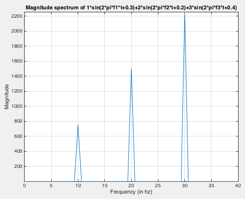
In the above code, we plotted wave containing three frequencies.

We have modelled the wave in which each frequency is travelling with the same velocity. We can add some complexity where every frequency in our wave is travelling with different speed. This is popularly known as dispersion.

Let us model our waves such that the wave speed for 1,2 and 3 Hz is 0.5,1 and 2 km/s.

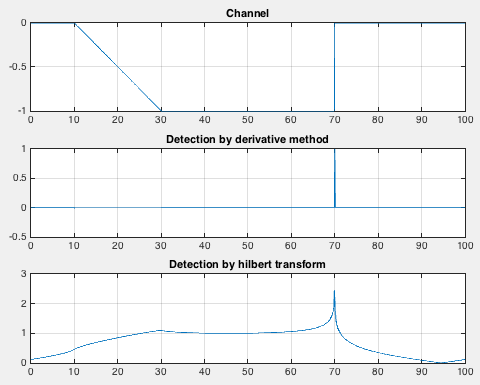
In this case, we can notice that the waves are travelling in groups and its shape keep changing.

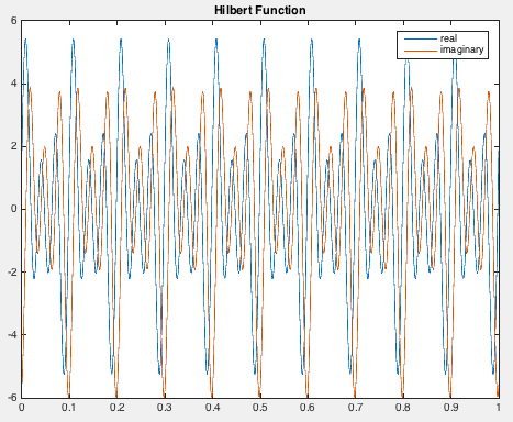
We can use the concept of hilbert transform to model the propagation of the group.

 

Modelling Waves (MATLAB)

We can use waves to model almost everything in the world from the thing we can see or touch to the things which we can’t.

Here, we try to model the waves itself.

Moving Waves

clear; close all; clc

a=1;    %amplitude

f=5;    %frequency

T=1/f;  %time period

w=2*pi*f;   %angular frequency

lb=2*T; %wavelength

k=2*pi/lb; %wavenumber

x=0:pi/200:10*pi;

t=0:0.01:2; %time

figure(1)

for i=1:length(t)

    y=a*sin(k*x-w*t(i));    %waveform

    plot(x,y)

    pause(0.1)

end

Fourier Transform to analyse the amplitude spectrum

clear; close all; clc

fs=1000;    %sampling frequency

t=0:1/fs:1.5-1/fs;%time

f1=10;  %frequency1

f2=20;  %frequency2

f3=30;  %frequency3

%x=5*sin(2*pi*10*t+3);

x=1*sin(2*pi*f1*t+0.3)+2*sin(2*pi*f2*t+0.2)+3*sin(2*pi*f3*t+0.4);

plot(t,x)

figure(1)

grid on

xlabel('Time')

ylabel('Amplitude')

title('Plot of 2*sin(2*pi*f1*t+0.3)-3*sin(2*pi*f2*t+0.2)+5*cos(2*pi*f3*t+0.4)') 

X=fft(x);

fre=fs/length(t);

fre_hz=(0:length(t)/2-1)*fre;

X_mag=abs(X);   %X is complex

figure(2)

plot(fre_hz,X_mag(1:length(t)/2))

grid on

axis([0 40 -inf inf])

xlabel('Frequency (in hz)')

ylabel('Magnitude')

title('Magnitude spectrum of 5*sin(2*pi*10*t+3)')

Hilbert Transform and get the envelope of the waveform

clear; close all; clc

fs = 1e4;   %sampling frequency

t = 0:1/fs:1;   %time

f1=10;  

f2=20;

f3=30;

x=1*sin(2*pi*f1*t+0.3)+2*sin(2*pi*f2*t+0.2)+3*sin(2*pi*f3*t+0.4);

%x=5*sin(2*pi*10*t+3);

y = hilbert(x);

figure(1)

plot(t,real(y),t,imag(y))

% %xlim([0.01 0.03])

legend('real','imaginary')

title('Hilbert Function')

figure(2)

env=abs(y);

plot(t,x)

xlabel('Time')

title('Envelope')

hold on

plot(t,env)

legend('original','envelope')

 

Application of Hilbert Transform: Edge Detection and comparison with the classical derivative method

clear; close all; clc

x = 0:0.1:100;

y = channel(x,[10 30 70]);  %channel function to define a trapezoidal channel

plot(x,y)

figure(1)

subplot(311)

plot(x,y)

grid on

title('Channel')

subplot(312)

deriv =diff(y); %dervative of the channel

plot(x(2:end),deriv)

title('Detection by derivative method')

grid on

subplot(313)

hil = hilbert(y);   %hilbert transform of the channel

env=abs(hil);

plot(x,env)

grid on

title('Detection by hilbert transform')

 

Channel Function

 

• – Utpal Kumar, IES, Academia Sinica