Travel time curve calculation for spherical, isotropic, homogeneous Earth model

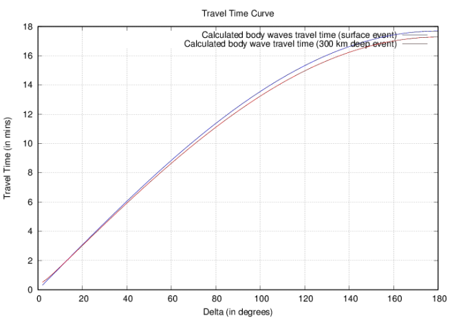
A travel time curve is a graph of the time it takes a seismic ray to reach the station from an earthquake versus the distance of the earthquake to the station (epicentral distance).

Here, we calculate the travel time curve for a spherically homogeneous Earth. This means the seismic velocity is constant for the whole earth. We have considered the three cases,

1. When the seismic ray travel through the body from the surface event to the station (body waves).
2. When the seismic ray for a deeper event (300 km depth) reaches the station.

Fortran code for calculation of the Model:

program travel_time_calc
    !Program to calculate seismic travel times in a spherical, homogeneous Earth.
    implicit none
    real, parameter :: pi = 2*asin(1.0), R = 6371    ! radius of Earth (km
    real :: V, xx, h1, h, dx
    integer, parameter :: n = 89
    integer :: i
    real(kind=16), allocatable, dimension(:) :: x, xrad, Di, Ti, Tim, Dhi, Thi, Thim

    V = 12;        ! assumed constant seismic wave velocity (km/s)
    dx=2 !increment
     allocate(x(0:n),xrad(0:n),Di(0:n),Ti(0:n),Tim(0:n),Dhi(0:n),Thi(0:n),Thim(0:n)) !allocating the size of the arrays
    write(*,*) "Distance (in degrees)", "  ","T-time surface (in mins)", "  ", "T-time interior (in mins)"
    open(1,file="Tcalc.dat")
    xx=0
    do i=0,n !do loop
        x(i) = xx + dx    !distance
        xrad(i) = x(i)*pi/180 ! convert degrees to radians
        !Path along the body
        Di(i) = 2*R*sin(0.5*xrad(i))    ! distance of the surface event along the body in km
        Ti(i) = Di(i)/V               ! travel time in seconds
        Tim(i) = Ti(i)/60             ! travel time in minutes
        
        !For deeper events (300 km)
        h1=300
        h=R-h1
        Dhi(i) = sqrt(R**2 + h**2 - 2*R*h*cos(xrad(i)))    !distance of the interior events in km
        Thi(i) = Dhi(i)/V                ! travel time in seconds
        Thim(i)= Thi(i)/60                ! travel time in minutes

         write(1,10) x(i), Tim(i), Thim(i) !printing output on the terminal
         write(*,10) x(i), Tim(i), Thim(i) !printing output on the terminal
        xx = x(i)
     end do
    10 format(f7.2, "  ",f8.4, "  ",f8.4)
    deallocate(x, xrad, Di, Ti, Tim, Dhi, Thi, Thim) ! deallocates the array
end program travel_time_calc

For the above program, we have considered the Earth to be isotropic and homogeneous with constant velocity of 12 km/s. Then we parameterize for 89 events each with 2 degrees interval from 2 to 180 degrees. The radius of the earth is assumed to be 6371 km.

For compiling and plotting (bash script):

#!/bin/bash

gfortran -ffree-form travel_time_calc.f -o travel_time_calc
./travel_time_calc

gnuplot << EOF
set terminal postscript color solid #terminal type
set title 'Travel Time Curve' #figure title
set xlabel 'Delta (in degrees)' #xlabel
set ylabel 'Travel Time (in mins)' #ylabel
set output 'travel_time.ps' #output fig name
set grid #grid
plot [:] [:] "Tcalc.dat" using 1:2 title "Calculated body waves travel time (surface event)" with lines lc rgb "blue", \
    "Tcalc.dat" using 1:3 title "Calculated body wave travel time (300 km deep event)" with lines lc rgb "red"
EOF

– Utpal Kumar (IES, Academia Sinica)

Understanding Seismograms

Seismograms are basic information about earthquakes, chemical and nuclear explosions, mining induced earthquakes, rock bursts and other events generating seismic waves.

Seismograms reflect the combined influence of the seismic source, the propagation paths, the frequency response of the recording instrument and the ambient noise at the recording site.

u(t) = s(t)*g(t)*i(t)*n(t).         “*” means convolution.

where, u is the seismic record, s is the source effect, g is the propagation effect, i is the instrument effect and n is the noise.

So, by understanding seismogram we can understand the seismic source, earth structure, and the noise in the medium.

This is our short attempt to understand the seismograms.

Understanding Seismograms 1

For understanding the seismogram, there are two main things we should notice- record duration and the dispersion. Due to different nature of the propagation velocity of the seismic waves and the different propagation paths taken by them to the station, travel time differences between the main group usually grows with distance. Since the body wave groups do not disperses, so their individual duration remains more or less constant, only the time difference between them changes with distance.

Figure 1: Event-Station Distribution map for the event in Mindanao, Phillipines Island (2005-02-05, Mw-7). The source is 540 km deep.

Figure 2

Figure 3

Figure 4

The epicentral distance for QIZ, BJT and DGAR is ~ 19, 35, 52 degrees respectively. For the station BJT (Figure 3), the epicentral distance is 35.2 degrees and for the station DGAR (Figure 4), the epicentral distance is 52.4 degrees. The P-S arrival times for the station BJT is nearly 300 sec and for the station DGAR, the P-S arrival time is nearly 400 sec. For the station QIZ, it is only around 200 sec. So, with the increase in epicentral distance, the difference in individual phase arrival increases. Also for the station DGAR, the P arrival is later than the BJT.

The time difference between main body wave onsets is:

Distance (degrees) less than	Time-difference in body wave onsets (P-S) in sec
10	180
60 (Fig 1,2,3)	960
100	1800
180	2700

Figure 5 : Travel-Time curve for depth 540 km

For the deep events, we do not see the first arrival as P wave (Figure 6) for short distances (D

Figure 6

Figure 6, is the seismogram at 2 degrees epicentral distance from the deep source. Here, we can notice that the first arrival is not P but the core reflected phase PcP. It is also cevident from the travel time curve(Figure 5).

Figure 7: Event-Station Distribution Map of Near Coast of Peru (2001-06-23, Mw-8.3). The source is at 2 km depth.

When the source is near the surface then we observe the surface waves as well in the seismogram.The surface waves from earthquakes at intermediate (> 70 km) or great depth (> 300 km) may have amplitudes smaller than those of body waves or may not even be detected on seismic records.

In contrast to the body waves, the velocity of surface waves is frequency dependent and hence it is dispersed. The duration of Love and Rayleigh waves increases with distance. As for station NNA (Figure 8), the duration of the first group of Rayleigh wave is about 230 seconds and for station HKT (Figure 9), the duration is around 600 seconds.

We can also notice that for shallower earthquake event, P-wave is the first arrival for stations less than 10 degrees of the source (Figure 10).

Figure 8

In Figure 8, we can notice that for surface waves, the largers periods arrive first than the lowers periods. This is the general case for normal layering. The larger periods sample the higher depths and since the velocity for higher depths is larger so it arrives before the shorter period waves.

Figure 9

In figure 9, for the surface waves, we can observe the wave groups or the beating effect (analogous to acoustics). This is because of the interference of the two or more harmonic waves with closer frequencies or periods.

Figure 10: Travel time curve for depth 2.2km

For certain distance ranges, the travel time curves for different types of seismic phases are close to each other or can even overlap (Figure 5,11).

(a)

(b)

 Figure 11: S, SKS and ScS are very close to each other.

The amplitude of P-wave depends not only on the epicentral distance but on the site effect (underground geology and crustal heterogeneity), azimuth etc.

The most obvious indication on a seismogram that a large earthquake has a deep focus is the small amplitude of the surface waves with respect to the body-wave amplitudes and the P and S waveforms often have impulsive onsets.

A more precise determination of the depth h of a seismic source, however, requires either the availability of a seismic network with at least one station being very near to the source, e.g., at an epicentral distance D < h (because only in the near range the travel time t(D, h) of the direct P wave varies strongly with source depth h), or the identification of seismic depthphases on the seismic record.

At distant seismograph stations, the depth phases pP or sP follow the direct P wave by a time interval that changes only slowly with distance but rapidly with depth.