Modelling Waves (MATLAB)

We can use waves to model almost everything in the world from the thing we can see or touch to the things which we can’t.

Here, we try to model the waves itself.

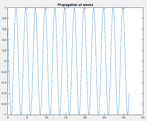
Moving Waves

clear; close all; clc

a=1;    %amplitude

f=5;    %frequency

T=1/f;  %time period

w=2*pi*f;   %angular frequency

lb=2*T; %wavelength

k=2*pi/lb; %wavenumber

x=0:pi/200:10*pi;

t=0:0.01:2; %time

figure(1)

for i=1:length(t)

    y=a*sin(k*x-w*t(i));    %waveform

    plot(x,y)

    pause(0.1)

end

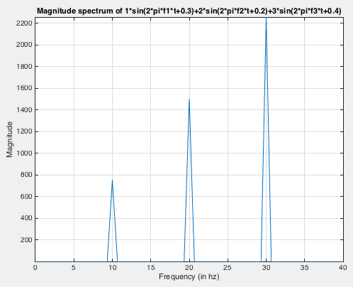
Fourier Transform to analyse the amplitude spectrum

clear; close all; clc

fs=1000;    %sampling frequency

t=0:1/fs:1.5-1/fs;%time

f1=10;  %frequency1

f2=20;  %frequency2

f3=30;  %frequency3

%x=5*sin(2*pi*10*t+3);

x=1*sin(2*pi*f1*t+0.3)+2*sin(2*pi*f2*t+0.2)+3*sin(2*pi*f3*t+0.4);

plot(t,x)

figure(1)

grid on

xlabel('Time')

ylabel('Amplitude')

title('Plot of 2*sin(2*pi*f1*t+0.3)-3*sin(2*pi*f2*t+0.2)+5*cos(2*pi*f3*t+0.4)') 

X=fft(x);

fre=fs/length(t);

fre_hz=(0:length(t)/2-1)*fre;

X_mag=abs(X);   %X is complex

figure(2)

plot(fre_hz,X_mag(1:length(t)/2))

grid on

axis([0 40 -inf inf])

xlabel('Frequency (in hz)')

ylabel('Magnitude')

title('Magnitude spectrum of 5*sin(2*pi*10*t+3)')

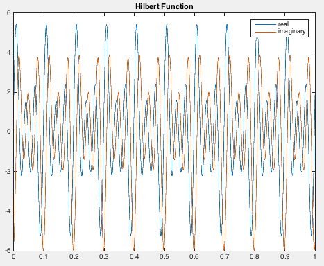
Hilbert Transform and get the envelope of the waveform

clear; close all; clc

fs = 1e4;   %sampling frequency

t = 0:1/fs:1;   %time

f1=10;  

f2=20;

f3=30;

x=1*sin(2*pi*f1*t+0.3)+2*sin(2*pi*f2*t+0.2)+3*sin(2*pi*f3*t+0.4);

%x=5*sin(2*pi*10*t+3);

y = hilbert(x);

figure(1)

plot(t,real(y),t,imag(y))

% %xlim([0.01 0.03])

legend('real','imaginary')

title('Hilbert Function')

figure(2)

env=abs(y);

plot(t,x)

xlabel('Time')

title('Envelope')

hold on

plot(t,env)

legend('original','envelope')

 

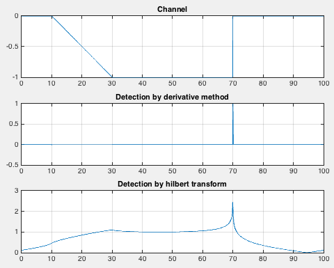
Application of Hilbert Transform: Edge Detection and comparison with the classical derivative method

clear; close all; clc

x = 0:0.1:100;

y = channel(x,[10 30 70]);  %channel function to define a trapezoidal channel

plot(x,y)

figure(1)

subplot(311)

plot(x,y)

grid on

title('Channel')

subplot(312)

deriv =diff(y); %dervative of the channel

plot(x(2:end),deriv)

title('Detection by derivative method')

grid on

subplot(313)

hil = hilbert(y);   %hilbert transform of the channel

env=abs(hil);

plot(x,env)

grid on

title('Detection by hilbert transform')

 

Channel Function

 

• – Utpal Kumar, IES, Academia Sinica

 

 

 

 

Seismic Resolution

Seismic resolution and fidelity are the two important measures of the quality of the seismic record and the seismic images. Seismic resolution quantifies the level of precision, such as the finest size of the subsurface objects detectable by the seismic data whereas the seismic fidelity quantifies the truthfulness such as the genuineness of the data or the level to which the imaged target position matches its true subsurface position.

Let us try to understand this by making a synthetic data and doing the analysis over it.

Seismic Resolution Analysis: 1

Estimation of the Width of the Fresnel’s Zone

The Fresnel’s resolution quantifies the resolvability of seismic wave perpendicular to the direction of wave propagation. Fresnel’s resolution is defined as the width of the first Fresnel’s zone due to interference of the spherical waves from the source and from the receiver.

Seismic Resolution Analysis: 2

Fidelity

To investigate the fidelity of our data, let us consider the technique of resampling. For our case we consider the method of “bootstrapping”. Bootstrapping basically relies on random sampling with replacement. The other popular method for resampling is “jackknifing” which predates “bootstrapping”. The jackknife estimator of a parameter is found by systematically leaving out each observation from a dataset and calculating the estimate and then finding the average of these calculations.

The principle behind “bootstrapping” is that a dataset is taken, the total dataset is divided into two by randomly sampling with replacement. The newly sampled data are now used to invert for the model using some kernel function. If the two models correlate high enough then we can say that the prominent features in the model come from consistent signals in the data.

We don’t have the data set to make the velocity model. So instead, we can take random Gaussian distribution data and play with it.

Let’s pose the null hypothesis that the two sets of data come from the same probability distribution (not necessarily Gaussian). Under the null hypothesis, the two sets of data are interchangeable, so if we aggregate the data points and randomly divide the data points into two sets, then the results should be comparable to the results obtained with the original data. So, the strategy is to generate random datasets, with replacement (bootstrapping), compute difference in means (or difference in medians or any other reliable statistic), and then compare the resulting values to the statistic computed from the original data.

Seismic Resolution Analysis: 3