Recently, we have joined hackathons and tried making web applications using Python. We intend to make tutorials on making these web apps. In this introduction, we present what we have done.
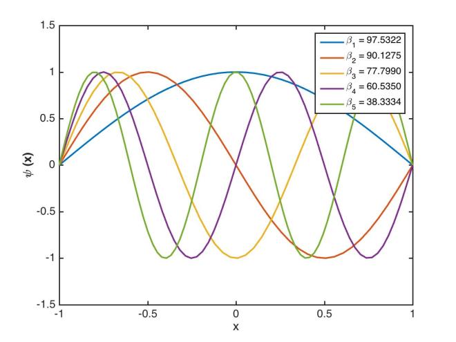
We are going to solve the differential equation with the boundary conditions
Let’s take the simpler boundary condition
.
Now, the first thing which we wanna do is to convert this equation in the first order form. After that, we can simply use the 4th order Runge-Kutta to obtain higher order solution.
To transform our 2nd order differential equation into first order, we define two variables. To transform nth order equations we need n such variables. This is the standard process to convert any differential equation into the system of first order differential equations.
Lets take
(1)
(2) [derivative of ]
So, we have transformed the 2nd order differential equation into two first order differential equations.
And our boundary condition will become
Now for the differential equations of the type
have the solution (for positive ). Now this solution doesn’t satisfy our condition . Exponential functions are monotonic and hence cannot be 0 at two points. So, this tells us that is not positive, i.e., .
Now, if , then our eqn becomes
The solution to this is of the form of cosines and sines, which has potential to satisfy the boundary condition. So, we have .
clear; close all; clcset(0,'defaultlinelinewidth',2);set(0,'defaultaxeslinewidth',1.5);set(0,'defaultpatchlinewidth',2);set(0, 'DefaultAxesFontSize', 14)tol=10^(-4); % define a tolerance level to be achieved% by the shooting algorithmxspan=[-1 1]; %boundary conditions % define the span of the computational domainA=1; % define the initial slope at x=-1ic=[0 A]; % initial conditions: x1(-1)=0, x1?(-1)=An0=100; % define the parameter n0dbeta=1;betasol=[];beta_start=n0; % beginning value of betafor jj=1:5 % begin mode loop beta=beta_start; % initial value of eigenvalue beta dbeta=n0/100; % default step size in beta for j=1:1000 % begin convergence loop for beta [t,y]=ode45('yfunc',xspan, ic,[],beta); % solve ODEs if y(end,1)*((-1)^(jj+1)) > 0 %this checks if the beta needs to be higher or lower for convergence beta = beta-dbeta; else beta = beta + dbeta/2; %uses bisection to converge to the solution dbeta=dbeta/2; end if abs(y(end,1)) < tol % check for convergence betasol=[betasol beta]; % write out eigenvalue break % get out of convergence loop end end beta_start=beta-0.1; % after finding eigenvalue, pick % new starting value for next mode norm=trapz(t,y(:,1).*y(:,1)); % calculate the normalization plot(t,y(:,1)/sqrt(norm)); hold onendbetasollegend(sprintf('\\beta_1 = %.4f',betasol(1)),sprintf('\\beta_2 = %.4f',betasol(2)),sprintf('\\beta_3 = %.4f',betasol(3)),... sprintf('\\beta_4 = %.4f',betasol(4)),sprintf('\\beta_5 = %.4f',betasol(5)));xlabel('x'); ylabel('\psi (x)','FontWeight','bold')saveas(gcf,'DiffEqnSol','jpg')
To find a basic introduction of GA, the first part can be found here.
III. Examples using Genetics Algorithm
In these examples, we will use Matlab and its function ga to apply GA for the optimization problem. For the manual of using this function, you can find it at https://www.mathworks.com/help/gads/ga.html or type in Matlab:
help ga
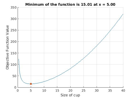
III.1. Optimization of a polynomial function
Problem: find the integer x value that minimizes function:
y = 0.2x2 + 50/x
First, we define the function:
function y = simple_fitness(x)
 y = 0.2*x.^2+(50./x);
And use Matlab to finish the job:
clear; close all; clc

x=linspace(0,40,100);
y=simple_fitness(x);
plot(x,y);

rng(1,'twister') % for reproducibility
lb=[1];
[x,fval] = ga(@simple_fitness,1,[],[],[],[],lb

xlabel('Size of cup');
ylabel('Objective Function Value');
title(sprintf('Minimum of the function is %.2f at x = %.2f',min(y), x))
grid on
And here is the result:
III.2. Find the best location of the earthquakes
Problem: we have a set of 5 seismic stations with coordinates: [-2 3 0; 1 3 0; -2 -1 0; 0 -3 0; 2 -2 0]
The travel time of seismic ray from EQ to stations is calculated from:
In daily life as well as in doing research, we might come to problems that require a lowest/highest value of variables, e.g.: find the shortest way from home to work, buying household items with a fixed amount of money, etc. These problems could be called “optimization” and today we will introduce an algorithm to solve these kinds of problem: the Genetic Algorithm.
Genetic Algorithm has been developed by Prof. John Holland in 1975, which search algorithm that mimics the process of evolution. This method is based on the “Survival of the Fittest” concept (Darwinian Theory), i.e.: successive generations are becoming better and better.
II. Algorithm
Initialization
Fitness Calculation
Selection
Crossing Over
Mutation
Repetition of the steps from 2-5 for the new population generated.
The pdf version of this introduction could be found here: Genetic Algorithm
In Earth Science research, sometimes we need to construct 3D surfaces from given points, for example: creating the fault surface, locating a subducting slab from earthquake hypocenters, etc. in a region of interest in X-Y plane.
In this example, we will show how to create a best-fit quadratic surface from given points in 3D using Matlab. The code is written in the following steps:
Input the data 3D points: x, y, z
Calculate the best fitting curve, store the parameters in C matrix.
Define a region of interest xx, yy and using C to get zz.
Plot the xx, yy, zz surface with x, y, z data.
Make comparison (probabilistic density function of misfit between z and zz).
% We start with some some 3d points
data = mvnrnd([0 0 0], [1 -0.5 0.8; -0.5 1.1 0; 0.8 0 1], 50);

x = data(:,1); y = data(:,2); z = data(:,3);


% Make a best-fit quadratic curve from the given points
C = x2fx(data(:,1:2), 'quadratic') \ data(:,3);


% Define an area of interest in X-Y plane by polyon nodes
xv = [-3 -3 0 3 3 0];
yv = [ 0 3 3 0 -3 -3];

% Create a area of interest in x, y plane
inpoints = getPolygonGrid(xv, yv, 1/0.1);
xx = inpoints(:,1);
yy = inpoints(:,2);

% Create the corresponding zz value from the above grid
zz = [ones(numel(xx),1) xx(:) yy(:) xx(:).*yy(:) xx(:).^2 yy(:).^2] * C;
zz = reshape(zz, size(xx));


% plot points and surface
figure('Renderer','opengl')
hold on;

% Plot the points
line(data(:,1), data(:,2), data(:,3), 'LineStyle','none', 'Marker','.', 'MarkerSize',25, 'Color','r')

% Make a triangular surface plot from xx, yy, zz
tri = delaunay(xx,yy); %x,y,z column vectors
trisurf(tri,xx,yy,zz, 'FaceColor','interp', 'EdgeColor','b', 'FaceAlpha',0.2);

% Change view propeties
title('Fitting surface');
grid on; axis tight equal;
view(9,9);
xlabel x; ylabel y; zlabel z;
colormap(cool(64))

% Calculate the misfit between surface and each points:
zfit = [ones(numel(x),1) x y x.*y x.^2 y.^2] * C;
h = -2: 0.01: 2;
misfit = z - zfit;
mu = mean(misfit); sigma = std(misfit);
f = exp(-(h-mu).^2./(2*sigma^2))./(sigma*sqrt(2*pi));
figure
title('Probability function of misfit');
hold on
plot(h,f,'LineWidth',1.5)
Earthquake location problem is old, however, it is still quite relevant. The problem can be stated as to determine the hypocenter (x0,y0,z0) and origin time (t0) of the rupture of fault on the basis of arrival time data of P and S waves. Here, we have considered hypocenter in the cartesian coordinate system. It can be readily converted to geographical coordinates using appropriate conversion factor. The origin time is the start time of the fault rupture.
Here, our data are the P and S arrival times at the stations located at the surface (xi,yi,0). We have also assumed a point source and a constant velocity medium for the simplicity sake.
The arrival time of the P or S wave at the station is equal to the sum of the origin time of the earthquake and the travel time of the wave to the station.
The arrival time, ti=Ti + t0, where Ti is the travel time of the particular phase and t0 is the origin time of the earthquake.
Ti = sqrt((xi-x0)^2 + (yi-y0)^2 + z0^2)/v; where v is the P or S wave velocity.
Now, we have to determine the hypocenter location and the origin time of the Earthquake. This problem is invariably ill-posed as the data are contaminated by noise. So, we can pose this problem as an over-determined case. One way to solve this inconsistent problem for the hypocenter and origin time is to minimize the least square error of the observed and predicted arrival times at the stations.
Before that, we need to formulate the problem. As evident from the above equation, the expression for arrival time and eventually the least square error function is nonlinear. This nonlinear inverse problem can be solved using the Newton’s method. We will utilize the derivative of the error function in the vicinity of the trial solution (initializing the problem with the initial wise guess) to devise a better solution. The next generation of the trial solution is obtained by expanding the error function in a Taylor series about the trial solution. This process continues until the error function becomes considerably small. Then we accept that trial solution as the estimated model parameters.
d = G m, where d is the matrix containing the arrival time data, m is the matrix containing the model parameters and G is the data kernel which maps the data to the model.
There are some instances where the matrix can become underdetermined and the least square would fail such as when the data contains only the P wave arrival times. In such cases the solution can become nonunique. We solve this problem as a damped least square case. Though it can also be using the singular value decomposition which allows the easy identification of the underdetermined case and then partitioning the overdetermined and underdetermined in upper and lower part of the kernel matrix and dealing with both part separately.
m = [G’G + epsilon]G’d
The parameter epsilon is chosen by trial and error to yield a solution that has reasonably small prediction error.
In this problem, we deduce the gradient of the travel time by examining the geometry of the ray as it leaves the source. If the earthquake is moved a small distance s parallel to the ray in the direction of the receiver, then the travel time is simply decreased by s/v, where v is the velocity of the phase. If the earthquake is moved a small distance perpendicular to the ray, then the change in travel time is negligible since the new path will have nearly same length as the old one.
T = r/v
If the earthquake is moved parallel to the ray path,
T” = (r-s)/v = r/v – s/v
delta T = T” – T = r/v – s/v – r/v = – s/v
If the earthquake has moved perpendicular to the raypath,
delta T = 0
So, delta T = – s/v, where s is a unit vector tangent to the ray at the source and points toward the receiver.
This is the Geiger’s Method, which is used to formulate the data kernel matrix.
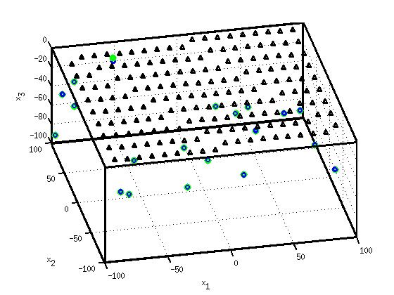
Let us take a hypothetical earthquake location problem and solve it using this method.
MATLAB Codes:
clear; close all;global G epsilon;
epsilon=1.0e-6;% Velocity parametersvpvs = 1.78;vp=6.5;vs=vp/vpvs;% defining the region of the problem which contains both the source and the receiver%We take a 100x100 units^2 area and the depth of 100 units. The surface is 0 units depth.
xmin=-100;xmax=100;ymin=-100;ymax=100;zmin=-100;zmax=0;
% stations: x, y, z coordinates (xi, yi, 0)sxm = [-9, -8, -7, -6, -5, -4, -3, -2, -1, 0, 1, 2, 3, 4, 5, 6, 7, 8, 9]'*ones(1,9)*10;sym = 10*ones(9,1)*[-9, -8, -7, -6, -5, -4, -3, -2, -1, 0, 1, 2, 3, 4, 5, 6, 7, 8, 9];sx = sxm(:);sy = sym(:);Ns = length(sx); % num of stationssz = zmax*ones(Ns,1); %zeros
% true earthquakes locations
Ne = 20; % number of earthquakes
M = 4*Ne; % 4 model parameters, x, y, z, and t0, per earthquake
extrue = random('uniform',xmin,xmax,Ne,1); %x0
eytrue = random('uniform',ymin,ymax,Ne,1); %y0
eztrue = random('uniform',zmin,zmax,Ne,1); %z0
t0true = random('uniform',0,0.2,Ne,1); %t0
mtrue = [extrue', eytrue', eztrue', t0true']'; %column matrix containing all the true model parameter values
Nr = Ne*Ns; % number of rays, that is, earthquake-stations pairs
N = 2*Ne*Ns; % total data; Ne*Ns for P and S each
% Generating the true data based on the true earthquake and station locations
dtrue=zeros(N,1); %allocating space for all data
for i = [1:Ns] % loop over stations
for j = [1:Ne] % loop over earthquakes
dx = mtrue(j)-sx(i); % x component of the displacement obtained by the difference between station and source location x component
dy = mtrue(Ne+j)-sy(i); % y component of the source- receiver displacement
dz = mtrue(2*Ne+j)-sz(i); % z component of displacement between source and receiver
r = sqrt( dx^2 + dy^2 + dz^2 ); % source-receiver distance
k=(i-1)*Ne+j;
dtrue(k)=r/vp+mtrue(3*Ne+j); %P arrival time for each station-source pair obtained by summing the travel time with the origin time of the earthquake
dtrue(Nr+k)=r/vs+mtrue(3*Ne+j); % S arrival time
end
end
% Generating observed data by adding gaussian noise with standard deviation 0.2
sd = 0.2;
dobs=dtrue+random('normal',0,sd,N,1); % observed data
%% Determining the predicted arrival time using the Geiger's Method
% inital guess of earthquake locations
mest = [random('uniform',xmin,xmax,1,Ne), random('uniform',ymin,ymax,1,Ne), ...
random('uniform',zmin+2,zmax-2,1,Ne), random('uniform',-0.1,0.1,1,Ne) ]';
% Here, we take a random initial guess
%Formulating the data kernel matrix and estimating the predicted models
for iter=[1:10] %for 10 iterations (termination criteria)
% formulating data kernel
G = spalloc(N,M,4*N); %N- total num of data,2*Ne*Ns; M is total num of model
%parameters, 4*Ne
dpre = zeros(N,1); %allocating space for predicted data matrix
for i = 1:Ns % loop over stations
for j = 1:Ne % loop over earthquakes
dx = mest(j)-sx(i); % x- component of displacement obtained using the initial guess
dy = mest(Ne+j)-sy(i); % y- component of displacement
dz = mest(2*Ne+j)-sz(i); % z- component of displacement
r = sqrt( dx^2 + dy^2 + dz^2 ); % source-receiver distance for each iteration
k=(i-1)*Ne+j; %index for each ray
dpre(k)=r/vp+mest(3*Ne+j); %predicted P wave arrival time
dpre(Nr+k)=r/vs+mest(3*Ne+j); %predicted S wave arrival time
%First half of data kernel matrix correspoding to P wave
G(k,j) = dx/(r*vp); % first column of data kernel matrix
G(k,Ne+j) = dy/(r*vp); % second column of data kernel matrix
G(k,2*Ne+j) = dz/(r*vp); % third column of data kernel matrix
G(k,3*Ne+j) = 1; % fourth column of data kernel matrix
% Second half of the data kernel matrix corresponding to S wave
G(Nr+k,j) = dx/(r*vs);
G(Nr+k,Ne+j) = dy/(r*vs);
G(Nr+k,2*Ne+j) = dz/(r*vs);
G(Nr+k,3*Ne+j) = 1;
end
end
% solve with dampled least squares
dd = dobs-dpre;
dm=bicg(@dlsfun,G'*dd,1e-5,3*M); solving using the biconjugate method
%solving the damped least square equation G'dd = [ G'G + epsilon* I] dm
% We use biconjugate method to reduce the computational cost (see for the dlsfun at the bottom)
mest = mest+dm; %updated model parameter
end
% Generating the final predicted data
dpre=zeros(N,1);
for i = 1:Ns % loop over stations
for j = 1:Ne % loop over earthquakes
dx = mest(j)-sx(i);
dy = mest(Ne+j)-sy(i);
dz = mest(2*Ne+j)-sz(i);
r = sqrt( dx^2 + dy^2 + dz^2 );
k=(i-1)*Ne+j;
dpre(k)=r/vp+mest(3*Ne+j); % S-wave arrival time
dpre(Nr+k)=r/vs+mest(3*Ne+j); % P- wave arriavl time
end
end
% Calculating the data and model misfit
expre = mest(1:Ne); % x0
eypre = mest(Ne+1:2*Ne); %y0
ezpre = mest(2*Ne+1:3*Ne); %z0
t0pre = mest(3*Ne+1:4*Ne); %t0
dd = dobs-dpre; %residual of observed and predicted arrival time
E = dd'*dd; %error
fprintf('RMS traveltime error: %f\n', sqrt(E/N) );
Emx = (extrue-expre)'*(extrue-expre); %misfit for x0
Emy = (eytrue-eypre)'*(eytrue-eypre); %misfit for y0
Emz = (eztrue-ezpre)'*(eztrue-ezpre); %misfit for z0
Emt = (t0true-t0pre)'*(t0true-t0pre); %misfit for t0
fprintf('RMS model misfit: x %f y %f z %f t0 %f\n', sqrt(Emx/Ne), sqrt(Emy/Ne), sqrt(Emz/Ne), sqrt(Emt/Ne) );
Earthquake location Example (William Menke, 2012) : The black triangles are the station locations, green circles are true earthquake location and the blue circles are predicted earthquake location.
dlsfun.m:
function y = dlsfun(v,transp_flag)global G epsilon;temp = G*v;y = epsilon * v + G'*temp;return
Refer to Chapter 5, Introduction to Seismology, Shearer 2009.
Problem:
From the P-wave travel time data below (note that the reduction velocity of 8km/s), inverse for the 1D velocity model using T(X) curve fitting (fit the T(X) curve with lines, then invert for the ray parameter p and delay time τ(p), then solve for the velocity and depth).
Fig 1. P-wave travel time from a seismic experiment.
Solution:
We construct the T(X) plot from the data: y = T – X/8 => T = y + X/8 and then divide the T(X) curve into fitting lines (Fig. 2).
Fig 2. T(X) plot with lines fitting to data points.
The ray parameter and delay is calculated for each line by using:
p = dT/dX
τ = T – pX
These parameters p and τ are slope and intercept of a line, respectively.
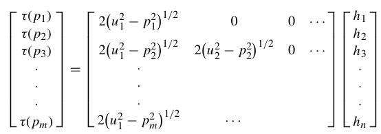
The τ(p) can be written as:
as in the matrix form of:
or, in short,
We can invert for the thickness of each layer using least square inversion:
If we assume ray slowness u(i) = p(i) for each line, we can solve the h and v for the 1D velocity model.
Here is the result of the inversion:
The sharp increase in Vp from ~6.6 km/s to 7.7 km/s at ~ 30km depth suggest for the Moho discontinuity.
Refer to Chapter 4 of Shearer, Introduction to Seismology.
For a ray piercing through Earth, the ray parameter (or horizontal slowness) p is defined by several expressions:
where u = 1/v is the slowness, θ is the ray incidence angle, T is the travel time, X is the horizontal range and utp is the slowness at the ray turning point.
The vertical slowness is defined as:
and integral expressions for the surface-to-surface travel time are:
With these equations we can calculate the travel time (T) and horizontal distance (X) for a given ray with ray parameter p and velocity model v(z).
Apply these to a problem (Exercise 4.8 Shearer):
(COMPUTER) Consider MARMOD, a velocity-versus-depth model, which is typical of much of the oceanic crust (Table 4.1). Linear velocity gradients are assumed to exist at intermediate depths in the model; for example, the P velocity at 3.75 km is 6.9 km/s. Write a computer program to trace rays through this model and produce a P-wave T(X) curve, using 100 values of the ray parameter p equally spaced between 0.1236 and 0.2217 s/km. You will find it helpful to use subroutine LAYERXT (provided in Fortran in Appendix D and in the supplemental web material as a Matlab script), which gives dx and dt as a function of p for layers with linear velocity gradients. Your program will involve an outer loop over ray parameter and an inner loop over depth in the model. For each ray, set x and t to zero and then, starting with the surface layer and proceeding downward, sum the contributions, dx and dt, from LAYERXT for each layer until the ray turns. This will give x and t for the ray from the surface to the turning point. Multiply by two to obtain the total surface-to-surface values of X(p) and T(p). Now produce plots of: (a) T(X) plotted with a reduction velocity of 8 km/s, (b) X(p), and (c) τ(p). On each plot, label the prograde and retrograde branches. Where might one anticipate that the largest amplitudes will occur?
Using the LAYERXT subroutine (Appendix D of Shearer), the FORTRAN and MATLAB can be downloaded from here. In this example, we will use python to calculate and plot the result.
The main program is as follow:
from ttcal import layerxt
import pandas as pd
import numpy as np
import matplotlib.pyplot as plt

v_model = pd.read_csv('v_model.dat')

p1 = 0.1236
p2 = 0.2217
n = 100

result = [['p','X','T']]
for p in np.linspace(p1, p2, n):
    X = 0; T = 0;
    for i in range(0, len(v_model)-1):
            p = p
            h = v_model.h[i+1] - v_model.h[i]
            utop = 1/v_model.vp[i]
            ubot = 1/v_model.vp[i+1]
            dx, dt, irtr = layerxt(p,h,utop,ubot)
            X += dx; T += dt
        #If the ray reflected at layer the dx, dt calculation stops
            if irtr == 2:
                    break
        result.append([p,X,T])

result_df = pd.DataFrame(result, columns=result.pop(0))
result_df = result_df[::-1]

#Multiply by 2 to get total surface-to-surface value ot X(p) and T(p)
result_df['T'] = 2*result_df['T']
result_df['X'] = 2*result_df['X']

plt.figure(1)
result_df['RT'] = result_df['T']-result_df['X']/8
result_df.plot(x='X', y='RT', legend=False)
plt.title('Reduction time')
plt.ylabel('Reduce time T - X/8 (s)')
plt.xlabel('Distance (km)')
plt.text(20,0.80,'Prograde', rotation =40)
plt.text(40,1.6,'Retrograde', rotation =35)
plt.text(80,1.00,'Prograde', rotation =0)
plt.savefig('ex4.8.1.png')

plt.figure(2)
result_df.plot(x='p', y='X', legend=False)
plt.title('X(p)')
plt.ylabel('Distance X (km)')
plt.xlabel('Ray parameter (km/s)')
plt.xlim([p1,p2])
plt.savefig('ex4.8.2.png')

plt.figure(3)
result_df['Taup'] = result_df['T'] - result_df['p']*result_df['X']
result_df.plot(x='p', y='Taup', legend=False)
plt.title('Tau(p)')
plt.ylabel('Tau(p) (s)')
plt.xlabel('Ray parameter (km/s)')
plt.xlim([p1,p2])
plt.savefig('ex4.8.3.png')

plt.figure(4)
v_model.h = v_model.h * (-1)
v_model.plot(x='vp', y='h', legend=False)
plt.ylabel('Depth (km)')
plt.xlabel('Velocity (km/s)')
plt.xlim([4,9])
plt.ylim([-10,0])
plt.savefig('ex4.8.4.png')

#plt.show()
LAYERXT subroutine written in python:
from math import sqrt, log


def layerxt(p,h,utop,ubot):
    ''' LAYERXT calculates dx and dt for ray in layer with linear velocity gradient

        Inputs:   p     =  horizontal slowness
             h     =  layer thickness
             utop  =  slowness at top of layer
             ubot  =  slowness at bottom of layer
        Returns:  dx    =  range offset
             dt    =  travel time
             irtr  =  return code
                   = -1,  zero thickness layer
                   =  0,  ray turned above layer
                   =  1,  ray passed through layer
                   =  2,  ray turned within layer, 1 segment counted in dx,dt'''
# ray turned above layer
    if p >= utop:
        dx = 0
        dt = 0
        irtr = 0
        return dx,dt,irtr

#Zero thickness layer
    elif h == 0:
        dx = 0
        dt = 0
        irtr = -1
        return dx,dt,irtr

#Calculate some parameters
    u1 = utop
    u2 = ubot
    v1 = 1.0/u1
    v2 = 1.0/u2
#Slope of velocity gradient
    b = (v2 - v1)/h
    eta1 = sqrt(u1**2 - p**2)

#Constant velocity layer
    if b == 0:
        dx = h*p/eta1
        dt = h*u1**2/eta1
        irtr = 1
        return dx,dt,irtr

    x1 = eta1/(u1*b*p)
    tau1=(log((u1+eta1)/p)-eta1/u1)/b

#Ray turned within layer, no contribution to integral from bottom point
    if p >= ubot:
        dx = x1
        dtau = tau1
        dt = dtau + p*dx
        irtr = 2
        return dx,dt,irtr

        irtr=1
    eta2=sqrt(u2**2-p**2)
    x2=eta2/(u2*b*p)
    tau2=(log((u2+eta2)/p)-eta2/u2)/b

    dx=x1-x2
    dtau=tau1-tau2

    dt=dtau+p*dx
    return dx,dt,irtr

def flat(zsph,vsph):
    ''' Calculate the flatten transformation from a spherical Earth.
        zf, vf = flat(zsph,vsph)'''

# Radius of the Earth
    a = 6371.0

    rsph = a - zsph
    zf = -a*log(rsph/float(a))
    vf = (a/float(rsph))*vsph
    return zf, vf
You need to install numpy, pandas and matplotlib package to run this. Normally it can be installed in the terminal by (presume python has been installed):


![\psi_{xx} +[100 - \beta ]\psi = 0](https://s0.wp.com/latex.php?latex=%5Cpsi_%7Bxx%7D+%2B%5B100+-+%5Cbeta+%5D%5Cpsi+%3D+0&bg=ffffff&fg=333333&s=0&c=20201002)
![\implies \psi_{xx} = [\beta - 100] \psi](https://s0.wp.com/latex.php?latex=%5Cimplies+%5Cpsi_%7Bxx%7D+%3D+%5B%5Cbeta+-+100%5D+%5Cpsi&bg=ffffff&fg=333333&s=0&c=20201002)
 .
. (1)
(1)

 (2) [derivative of
  ]
]
![\implies y_2' = [\beta - 100] \psi](https://s0.wp.com/latex.php?latex=%5Cimplies+%C2%A0y_2%27+%3D+%5B%5Cbeta+-+100%5D+%5Cpsi+&bg=ffffff&fg=333333&s=0&c=20201002)

![\psi_{xx} = [\beta - 100] \psi](https://s0.wp.com/latex.php?latex=%5Cpsi_%7Bxx%7D+%3D+%5B%5Cbeta+-+100%5D+%5Cpsi&bg=ffffff&fg=333333&s=0&c=20201002)

 (for positive
  ). Now this solution doesn’t satisfy our condition
  .
. , then our eqn becomes