Generic Mapping Tool (GMT) for Beginners

To download all the scripts, figures and data, click here.

Basemap for Linear Plots:


Bash script to generate above plots is here.

Plotting Maps:

Bash script to generate above plots is here and here.

Writing Text on the Figure:

GMT_figure14

Bash script to generate above plots is here.

Contour Plots:

Bash script to generate above plots is here.

Colored Images and Color-bars:

Bash script to generate above plots is here.

3-D Plots:

GMT_figure24GMT_figure23

Bash script to generate above plots is here.


Cross Section for Oblique Projection Problem

Sometimes, to create a cross section profile is not that easy when it comes to an Oblique projection map. Maybe, not only that, to make a cross section profile is not that easy either when it comes to various direction of cross section lines, which in most cases we try to fed up our interest and gives a reasonable view to convince other people ‘the reader’ about our finding.

Traditionally, if the cross section is parallel to the latitude then we can select the longitude values in degree as the distance along the cross section profile (this maybe worth to try for the case in Taiwan). This is not the case when it comes to an oblique projection plot, or random cross section directions. The latitude and longitude may vary along the cross section line. Here is the problem, how we can make a cross section that depends on the distance along the profile?

In this way you guys may understood that this post not only for the oblique projection problem, but you may try to a traditional case (North-South & East-West map projection orientation) and make a different cross sectional direction.

To do this, GMT provide a command that allow us to select a data along the profile which indicated by a starting and ending point  longitude and latitude information, respectively.

The files that you need are the same as the one that we post for oblique projection problem. You may try the GMT script as follow:

#!/bin/bash
#environment setting
#######################################################################
gmtset PAPER_MEDIA A3
gmtset LABEL_FONT_SIZE = 12p
gmtset BASEMAP_TYPE plain
gmtset ANNOT_FONT_SIZE_PRIMARY = 12p
gmtset ANNOT_FONT_SIZE_SECONDARY = 12p
gmtset HEADER_FONT_SIZE = 14p

#######################################################################
########################Parameters#####################################
####################change start here##################################
####topographic file####
inputgrd=sumatra1.grd

####range and projection for regional map####
range1=95/-2/97/8r
oblq1=98.5/4/55/4i

####range and projection for study area map####
range2=96/-1/95.95/5r
oblq2=100/10/10/54/5.8i

####cpt, gradient and trench####
makecpt -Crelief -T-8500/3500/500 -Z -V > sumatra.cpt
makecpt -Ccyclic -T0/50/1 -Z -V > eventdepth.cpt 
mapcpt=sumatra.cpt
inputgradient=sum1_intens.grd
trench=sumatra_trench.clip
eventcpt=eventdepth.cpt

####catalog data####
usgscat=usgs_cat2005.dat
datafiles=(m4_2005.xyz m5_2005.xyz m6_2005.xyz m7_2005.xyz m8_2005.xyz)

####cross section####
#along y direction
maxdistx=`minmax bath_y1.xyz | awk '{print $7}' | awk -F/ '{print $2}' | awk -F">" '{print $1}'`
range3=0/$maxdistx/-50/5
startpointx=97/-0.3 
endpointx=94.15/3.65
position4='-X6.25i -Y2i'
widthx='-W-200/200'

#along x direction
maxdisty=`minmax bath_x1.xyz | awk '{print $7}' | awk -F/ '{print $2}' | awk -F">" '{print $1}'`
range4=-50/5/0/$maxdisty
startpointy=94.6/1 
endpointy=97.4/3
position3='-Y-2i'
widthy='-W-80/80'

####output####
output=oblique_subduction.ps
rm -f $output
#####################change end here###################################
#######################################################################
#######erthquake event from usgs cataloque custom area and time########
#magnitude 4 - 8
i1=4
i2=5
for i in {0..4}
do
awk -v i1=$i1 -v i2=$i2 '{if ($5>=i1 && $5<i2) print $3, $2, $4}' $usgscat > ${datafiles[$i]} 
(( i1 = i1 + 1 ))
(( i2 = i2 + 1 ))
done

#Eq ploting size#
mag=('-Sc0.04i' '-Sc0.07i' '-Sc0.10i' '-Sc0.15i' '-Sc0.25i')

#start, continue and end#
start='-K -V'
continue='-K -O -V'
end='-O -V'

#position for regional and study area map#
position1='-X11.7i -Y7.5i'
position2='-X-10i -Y-4.85i'

#######Map Script for regional map#######
#grd image#
grdgradient $inputgrd -A0/270 -G$inputgradient -Ne0.6 -V
grdimage $inputgrd -R$range1 -JOa$oblq1 -Ba1f0.5WNSE -C$mapcpt -I$inputgradient $position1 $start > $output

#coast line#
pscoast -R -J -B -Dh -W1.5p,black $continue >> $output

#costum contour line#
grdcontour $inputgrd -R -J -C500 -L-7000/-4500 $continue >> $output
grdcontour $inputgrd -R -J -C100 -L-4500/-3500 $continue >> $output

#sumatra_trench#
psxy $trench -R -B -J -Sf0.5i/0.1ilt -Gred -W0.03i,red $continue >> $output

#input event costum sized#
#magnitude 4
for i in {0..4}
do
psxy ${datafiles[$i]} -R -J ${mag[$i]} -W0.001p -C$eventcpt $continue >> $output
done

#make a rectangle indicate for the study area#
psxy -R -J -W0.02i/red $continue << EOF >> $output
95.95 5
93.20 2.98
96.1 -1
#> next (this gonna disconnect the points)#
98.8 1.01
95.95 5
EOF

#cross section line#
psxy -R -J -W0.02i,black $continue << END >> $output
94.6 1
97.4 3
END

#######Map Script for study area map#######
grdimage $inputgrd -R$range2 -JOc$oblq2 -Ba1f0.5WNSE -C$mapcpt -I$inputgradient $position2 $continue >> $output

#coast line#
pscoast -R -J -Dh -Ba1f0.5WNSE -W1.5p,black $continue >> $output

#costum contour line#
grdcontour $inputgrd -R -J -C500 -L-5000/-4500 $continue >> $output
grdcontour $inputgrd -R -J -C100 -L-4000/-1000 $continue >> $output
grdcontour $inputgrd -R -J -C250 -L-1000/-250 $continue >> $output

#input sumatra_trench
psxy $trench -R -B -J -Sf0.5i/0.1ilt -Gred -W0.03i,red $continue >> $output

#input event costum sized#
for i in {0..4}
do
psxy ${datafiles[$i]} -R -J ${mag[$i]} -W0.001p -C$eventcpt $continue >> $output
done

#######cross section line#######
psxy -R -J -W0.02i,black $continue << END >> $output
94.6 1
97.4 3
END

#project with start and end latitude 94.6 1 97.4 3#
project -C$startpointy -E$endpointy -G1 -Q | grdtrack -G$inputgrd > bath_y1.xyz

#project eq on horizontal line
inm=4
for i in {0..4}
do
project ${datafiles[$i]} -C$startpointy -E$endpointy -Fxyzpqrs -Lw $widthy -Q > ${inm}_ycross.dat
(( inm = inm + 1 ))
done

#insert depth event look from south to north
psbasemap -R$range3 -JX5.81i/1.5i -Ba50f10:"Distance (km)":/a10f5WnSe:"Depth (km)": -P $position3 $continue >> $output
awk '{print $3, $4/500}' bath_y1.xyz | psxy -R -JX -W3,black $continue >> $output

#projected earthquake event
inm1=4
for i in {0..4}
do
awk '{print $4, -$3, $3}' ${inm1}_ycross.dat | psxy -R -JX ${mag[$i]} -W0.00001p -Ceventdepth.cpt $continue >> $output
(( inm1 = inm1 + 1 ))
done

#project with start and end latitude 97 -0.394.15 3.65
project -C$startpointx -E$endpointx -G1 -Q | grdtrack -Gsumatra1.grd > bath_x1.xyz

#project eq on horizontal line
inm2=4
for i in {0..4}
do
project ${datafiles[$i]} -C$startpointx -E$endpointx -Fxyzpqrs -Lw $widthx -Q > ${inm2}_xcross.dat
(( inm2 = inm2 + 1 ))
done

#insert depth event look from west to east
psbasemap -R$range4 -JX-2i/8.1i -Ba50f10wNsE:"Depth (km)":/a100f50:"Distance (km)": -P $position4 $continue >> $output
awk '{print $4/500, $3}' bath_x1.xyz | psxy -R -JX -W3,black $continue >> $output

#projected earthquake event
inm3=4
for i in {0..3}
do
awk '{print -$3, $4, $3}' ${inm3}_xcross.dat | psxy -R -JX ${mag[$i]} -W0.00001p -Ceventdepth.cpt $continue >> $output
(( inm3 = inm3 + 1 ))
done

#closing the overlay
awk '{print -$3, $4, $3}' ${inm3}_xcross.dat | psxy -R -JX ${mag[4]} -W0.00001p -Ceventdepth.cpt $end >> $output

gv $output

After you execute the program, you may get a figure as shown below.

1


From the script above, most of the command line are the same as the previous post. Two things that you need to consider is that; 1st to make the cross section, which means that to select the data along the cross section line (i.e. starting to ending point) in a particular distance from the center of the profile, we use a GMT command ‘project‘.

Within the script above, we use this command in several purposes that I point out as follow:

  1. To select only longitude and latitude information along the profile. Then, we may use the result for the grdtrack. The grdtrack will extract the Z value from a grid file along a given longitude and latitude information (result that we get after project). As the result in the profile, you may see  a black line that indicate the bathymetry or topography.
  2. To convert the longitude and latitude information (unit degree) to distance (unit km). You may set it up in the -F option within the project, where the ‘p‘ indicate for the distance in km.
  3. To select the data coverage along the profile, which indicated by -Lw $widthx and $widthy, respectively. For this purpose, the project provide several options that you can choose. Here we present the project, to select the data along the cross section profile with a particular width respect to the center along the profile.

The 2nd thing that you need to consider is that, you need to check the maximum distance of the profile. You can easily know this by typing minmax bath_y1.xyz and bath_x1.xyz, respectively in your terminal (this minmax already done within the script at the cross section parameters). The distance should be appear at the 4th column (the ‘p‘ in -F). Then, you can set up your range for the cross section profile.

For next post, we will finally put the necessary information within our map to make it complete, such as legend, scale bar, and arrow for north direction.

  •                                  Haekal A. Haridhi, TIGP Program, IES, Academia Sinica

Using Generic Mapping Tool (GMT) for Oblique Projection Problem

In previous post (Using Generic Mapping Tool (GMT) Basic) we make a map with the study area is located at Taiwan, where the subduction trench are either having South-North and or West-East  orientations, respectively. For these subduction systems, we could make a cross section immediately perpendicular to the trench orientation, i.e. West-East (for the South-North oriented trench) and South-North (for the West-East orientated trench). From this cross section, we could see the Wadati-Benioff zone clearly from the earthquakes distribution (although clear or not will be depend on your data quality).

However, this not the case for the study area at Sumatra (Using Generic Mapping Tool (GMT) Basic II), where the subduction trench is Northeast-Southwest orientation or we can call it as an oblique subduction. If we make a cross section as same as the one that we described earlier, we wouldn’t able to see the Wadati-Benioff zone. Now this is the problem, how we could rotate the map so that it will have a parallel orientation to the trench?

For this problem, we could solve it easily by using the GMT. The GMT provide various map projection that enable us to plot a map in almost what ever orientation that we wanted to. Keep in mind that, in this post we work on a Linux Operating System (OS) with GMT version 4.5 (some features, i.e., to make a file executable, post script viewing (.ps) and others, you may need to change it or install some program in order to work and viewing the output).

For this post, the files that you need are listed as shown below (freely accessible).

  1. Topography grid file GEBCO 30-arc second (download here).
  2. Earthquake event (customized for this post only) at northern Sumatra region from the USGS earthquake catalog (download here).
  3. Sumatra trench file from the USGS (download here).
  4. Color file for the map (you can create by yourself, or download here).
  5. Color file for the earthquake event (same as number 4, or download here).

After you downloaded all the files, make sure that these files are located in the same folder as your scrip. Now, you may try to plot the Map by using this script as follow.

#!/bin/csh
#environment setting
gmtset PAPER_MEDIA A3
gmtset LABEL_FONT_SIZE = 12p
gmtset BASEMAP_TYPE plain
gmtset ANNOT_FONT_SIZE_PRIMARY = 12p
gmtset ANNOT_FONT_SIZE_SECONDARY = 12p
gmtset HEADER_FONT_SIZE = 14p

####topographic file####
set inputgrd=sumatra1.grd

####range and projection for regional map####
set range1=95/-2/97/8r
set oblq1=98.5/4/55/4i

####range and projection for study area map####
set range2=96/-1/95.95/5r
set oblq2=100/10/10/54/5.8i

####cpt, gradient and trench####
set mapcpt=sumatra.cpt
set inputgradient=sum1_intens.grd
set trench=sumatra_trench.clip
set eventcpt=eventdepth.cpt

####erthquake event from usgs cataloque custom area and time#####
#magnitude 4
awk '{if ($5>=4 && $5<5) print $3, $2, $4}' usgs_cat2005.dat > m4_2005.xyz 
#magnitude 5
awk '{if ($5>=5 && $5<6) print $3, $2, $4}' usgs_cat2005.dat > m5_2005.xyz
#magnitude 6
awk '{if ($5>=6 && $5<6) print $3, $2, $4}' usgs_cat2005.dat > m6_2005.xyz
#magnitude 7
awk '{if ($5>=7 && $5<8) print $3, $2, $4}' usgs_cat2005.dat > m7_2005.xyz
#magnitude 8
awk '{if ($5>=8 && $5<9) print $3, $2, $4}' usgs_cat2005.dat > m8_2005.xyz

####output####
set output=oblique_subduction.ps

####Map Script for regional map####

#grd image#
grdgradient $inputgrd -A0/270 -G$inputgradient -Ne0.6 -V
grdimage $inputgrd -R$range1 -JOa$oblq1 -Ba1f0.5WNSE -C$mapcpt -I$inputgradient -X11.7i -Y7.5i -K -V > $output

#coast line#
pscoast -R -J -B -Dh -W1.5p,black -O -K -V >> $output

#custom contour line#
grdcontour sumatra1.grd -R -J -C500 -L-7000/-4500 -K -O -V >> $output
grdcontour sumatra1.grd -R -J -C100 -L-4500/-3500 -K -O -V >> $output

#sumatra_trench#
psxy $trench -R -B -J -Sf0.5i/0.1ilt -Gred -W0.03i,red -K -O -V >> $output

#input event custom sized#
#magnitude 4
psxy m4_2005.xyz -R -J -Sc0.04i -W0.001p -C$eventcpt -K -O -V >> $output
#magnitude 5
psxy m5_2005.xyz -R -J -Sc0.07i -W0.001p -C$eventcpt -K -O -V >> $output
#magnitude 6
psxy m6_2005.xyz -R -J -Sc0.10i -W0.001p -C$eventcpt -K -O -V >> $output
#magnitude 7
psxy m7_2005.xyz -R -J -Sc0.15i -W0.001p -C$eventcpt -K -O -V >> $output
#magnitude 8
psxy m7_2005.xyz -R -J -Sc0.20i -W0.001p -C$eventcpt -K -O -V >> $output

#make a rectangle indicate for the study area#
psxy -R -J -W0.02i/red -K -O -V << EOF >> $output
95.95 5
93.20 2.98
96.1 -1
#> next (this gonna disconnect the points)#
98.8 1.01
95.95 5
EOF

#cross section line#
psxy -R -J -W0.02i,black -K -O -V << END >> $output
94.6 1
97.4 3
END

####Map Script for study area map####
grdimage $inputgrd -R$range2 -JOc$oblq2 -Ba1f0.5WNSE -C$mapcpt -I$inputgradient -X-9i -Y-4.3i -K -O -V >> $output

#coast line#
pscoast -R -J -Dh -Ba1f0.5WNSE -W1.5p,black -K -O -V >> $output

#custom contour line#
grdcontour sumatra1.grd -R -J -C500 -L-5000/-4500 -K -O -V >> $output
grdcontour sumatra1.grd -R -J -C100 -L-4000/-1000 -K -O -V >> $output
grdcontour sumatra1.grd -R -J -C250 -L-1000/-250 -K -O -V >> $output

#input sumatra_trench
psxy $trench -R -B -J -Sf0.5i/0.1ilt -Gred -W0.03i,red -K -O -V >> $output

#input event custom sized#
#magnitude 4
psxy m4_2005.xyz -R -J -Sc0.04i -W0.001p -C$eventcpt -K -O -V >> $output
#magnitude 5
psxy m5_2005.xyz -R -J -Sc0.07i -W0.001p -C$eventcpt -K -O -V >> $output
#magnitude 6
psxy m6_2005.xyz -R -J -Sc0.10i -W0.001p -C$eventcpt -K -O -V >> $output
#magnitude 7
psxy m7_2005.xyz -R -J -Sc0.15i -W0.001p -C$eventcpt -K -O -V >> $output
#magnitude 8
psxy m8_2005.xyz -R -J -Sc0.20i -W0.001p -C$eventcpt -K -O -V >> $output

#cross section line#
psxy -R -J -W0.02i,black -O -V << END >> $output
94.6 1
97.4 3
END

gv $output

After you execute the program, you may get a map as shown below.

1_3

Here are some explanations to the script:

  1. Oblique projection can be made by using range as described in set range1 and set range2, which are the range of the regional and study area maps respectively. If you see carefully, we append a small “r” later at the end of the range. This implies that we will use lower left corner and upper right corner longitude and latitude information for the map range.
  2. We use two types of oblique projection (you may type in the terminal man grdimage to get a full description):
    1. -JOa$oblq1” means that we will use a cylindrical projection with an Oblique Mercator – point and azimuth.
    2.  “-JOc$oblq2” same as 1, but with an Oblique Mercator – point and pole.
  3. We make the illuminations of the topography grid file by using grdgradient.
  4. We use a simple shell command such as awk, i.e. to get the preferred column being printed to the file that we want, such as the usgs_cat2005.dat being printed to a several files with different magnitude (column 5 in the .dat file indicate for the earthquake magnitude).
  5. We set up a custom earthquake size. In default, the psxy command will search the 4th column as the earthquake size and will plot the size using default size. However, we can customized the size that we want to see the earthquake with larger magnitude has a “logarithmic” size from the small one, so it will give us an “appealing” attention to the big magnitude event as the main shock.

Keep in mind that, this post only show how to rotate the map, not the cross section plot. However, we already make a line for the cross section and we will cover that for the next post.

  •                                  Haekal A. Haridhi, TIGP Program, IES, Academia Sinica

Using Generic Mapping Tool (GMT) Basic II

Continuing from the previous post about GMT, now we will cover some others code to produce a map, and also to get some data from the free available sources. To start it, we may try a very simple command to produce a map. Keep in mind that, in this post we work on a Linux Operating System (OS) with GMT version 4.5 (some features, i.e., to make a file executable, post script viewing (.ps) and others, you may need to change it or install some program in order to work and viewing the output).

Here is the idea: We want to produce a map that consist of considerably regional map and a study area within a single plot (one figure with two maps ~ or we can say it, as such as the famous “figure of study area”).

Well, there are couple of ways to do it so, and we will start again as we mention earlier as a very simple one. Here we go:

A. We will only use a pscoast command to make it. You may try it as follows:

 #!/bin/csh
 #environment setting
 gmtset PAPER_MEDIA A3
 gmtset LABEL_FONT_SIZE = 12p
 gmtset BASEMAP_TYPE plain
 gmtset ANNOT_FONT_SIZE_PRIMARY = 12p
 gmtset ANNOT_FONT_SIZE_SECONDARY = 12p
 gmtset HEADER_FONT_SIZE = 14p

###regional map
 pscoast -R95/102/-2/6 -JM4i -Ba1f0.5NSEw -Dh -W0.5p,black -X11.7i -Y6.8i -K -V > nearshore.ps

###study area map
 pscoast -R95.18/95.55/5.5/5.75 -JM10i -Ba0.05f0.01NSEW -Dh -W0.5p,black -X-11i -Y-6.5i -O -V >> nearshore.ps

gv nearshore.ps

After you write this code you may make it executable by:

1

After the program run, you may get a figure as shown below.

2

Now you get a figure as what we have in mind. Okay, now, I will try to explain the code that I wrote above so it will be meaningful for everyone. The explanation are as follows:

  1. The first line (LN) is a command for Linux to access the csh.
  2. LN 3-8 are some setting that I want to change for my gmt default (this is kind of personal stuff, so you may do it as what ever you want). You may check other options, just type in your terminal gmtdefaults -L to make a change or keep it, as that is based on your personal taste.
  3. LN 11 is the pscoast command that will plot you the regional map. the -R option gives you the range coverage of your map, -JM is your map projection (Mercator) with the size of 4i (i stand for inch), -Ba is your map annotation which shown the degree value (we set it to show the value in each 1 degree and in between we set a 0.5 degree as a small thick), and the NSEw will show you where you need to show the degree value (capital later) and no need to show it (small later). -D indicate the coast line resolution that you gonna use and h is high. Caution : you may check it first in your machine, is the high resolution coast line is available or not. You may check it by going to the root as is shown in figures below.3And then you may find4.pngIf you see something just like the one indicated by the red rectangle, then you already have the high resolution coast file installed in your machine. If it is not showing like that, then you only have the low resolution (please use -Dl). To install it, you may just yum install GMT-coastlines-high.noarch. Okay, we continue, -W will gives you the thickness of the coast line and we use 0.5p (p is point/pixel) and a comma sign (,) to gives the color (here we used a black color).-X and -Y were used to set the location of the map on the paper with (+) X and Y value will put your map to the right and up respectively, and opposite with (-) value. Here we want to put the regional map at the upper righthand side of the study area map. -K indicate that you will have another command after this line and -V is a verbose mode (report everything in terminal during the execution/ the program run). The greater then sign (>) will gives you the output and the output file name is nearshore.ps.
  4. LN 14 is the same thing as what we already explain in number 3, but here we make a smaller range (see the -R), make a larger size (see -JM), set up the location of the map on the paper (see -X and -Y), an additional of -O is to overlay this map with the previous one and two greater then symbols (>>) to print this map in the same output file as previous command.
  5. LN 16 is the ghost view command that will pop up the output file as soon as it is finish (to make your life easy).

Okay, we already got the figure, are we finish?not quiet. We can add the location of the study area in our regional map. This can be done by adding a psxy command after the first pscoast command. Now the GMT script is shown like this:

 #!/bin/csh
#environment setting
gmtset PAPER_MEDIA A3
gmtset LABEL_FONT_SIZE = 12p
gmtset BASEMAP_TYPE plain
gmtset ANNOT_FONT_SIZE_PRIMARY = 12p
gmtset ANNOT_FONT_SIZE_SECONDARY = 12p
gmtset HEADER_FONT_SIZE = 14p

###regional map
pscoast -R95/102/-2/6 -JM4i -Ba1f0.5NSEw -Dh -W0.5p,black -X11.7i -Y6.8i -K -V > nearshore.ps

###make a rectangle indicate for the study area
psxy -R -J -W0.01i/red -K -O -V << EOF >> nearshore.ps
95.18 5.5
95.55 5.5
95.55 5.75
#> next (this gonna disconnect the points)
95.18 5.75
95.18 5.5
EOF

###study area map
pscoast -R95.18/95.55/5.5/5.75 -JM10i -Ba0.05f0.01NSEW -Dh -W0.5p,black -X-11i -Y-6.5i -O -V >> nearshore.ps

gv nearshore.ps

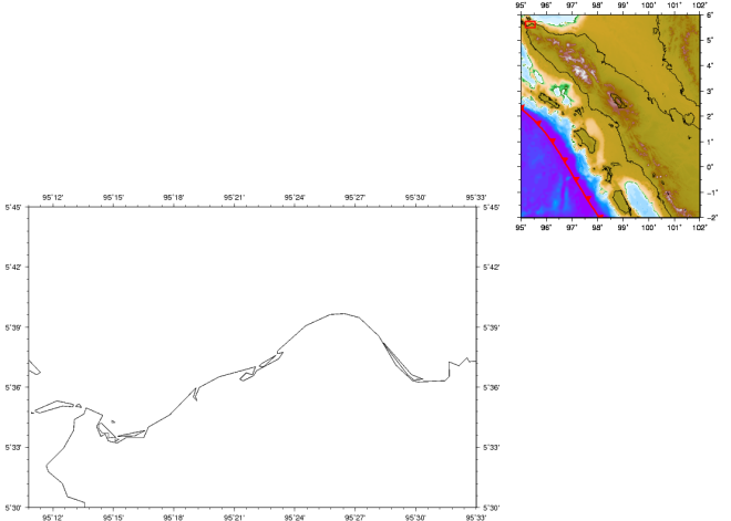
You may execute this program again and it will give you this figure:

5

If you see carefully there is a red rectangle at the upper left corner of the regional map (northern tip of Sumatra Island).

To make that rectangle see the ###make rectangle … The psxy command will plot a point on the map (first line below psxy, longitude (lon) and latitude (lat) information) and connect it to another point (second line, lon and lat) and so on. For this command we will follow the -R, -J of the previous command.

Now the information seems quiet complete. But, you may add some important information (tectonically), such as topography and  trench location. To do that, we revise this script, and now we go to B much more advance than A.

B. We will use a grid file (.nc or .grd) from the free available resources. Here we use a GEBCO 30-arc second in our map. You can just follow the instruction in  GEBCO website to get the .nc or .grd file. The other information that we need is a trench location (for a subduction area), the file is available at the USGS website and please see or follow the instruction which file that you need in your map at this website.

After you downloaded these two files, make sure that these files are located within the same folder as your .gmt script file located and please make sure that the grid file that you downloaded from GEBCO was using the same file name as well as the trench clip file, i.e. in the script below: gebco_1.nc and sumatra_trench.clip, respectively.

Now you may try to execute this script below.

#!/bin/csh
#environment setting
gmtset PAPER_MEDIA A3
gmtset LABEL_FONT_SIZE = 12p
gmtset BASEMAP_TYPE plain
gmtset ANNOT_FONT_SIZE_PRIMARY = 12p
gmtset ANNOT_FONT_SIZE_SECONDARY = 12p
gmtset HEADER_FONT_SIZE = 14p

###resample the grd file to fit in range of regional map
grdsample gebco_1.nc -Gsumatra.grd -R95/102/-2/6 -I0.005 -V

###set color for the grid file
makecpt -Cglobe -T-5775/3590/10 -Z -V > sumatra.cpt

###grd image 
grdimage sumatra.grd -R95/102/-2/6 -JM4i -Ba1f0.5NSEw -Csumatra.cpt -X11.7i -Y6.8i -K -V > nearshore.ps

###regional map
pscoast -R -JM -B -Dh -W0.5p,black -K -O -V >> nearshore.ps

###input sumatra_trench
psxy sumatra_trench.clip -R -B -J -Sf0.5i/0.1ilt -Gred -W0.03i,red -K -O -V >> nearshore.ps

###make a rectangle indicate for the study are
psxy -R -J -W0.03i/red -K -O -V << EOF >> nearshore.ps
95.18 5.5
95.55 5.5
95.55 5.75
#> next (this gonna disconnect the points)
95.18 5.75
95.18 5.5
EOF

###study area map
pscoast -R95.18/95.55/5.5/5.75 -JM10i -Ba0.05f0.01NSEW -Dh -W0.5p,black -X-11i -Y-6.5i -O -V >> nearshore.ps

gv nearshore.ps

After the program run, you may get a figure as shown below.

6

Now your regional map already have the topographic view and a trench location.

Using Generic Mapping Tool (Basics)

Generic Mapping Tool (GMT) is an open-source collection of commands for processing and displaying 2D or 3D datasets. It also has features like rasterization, filtering and other image processing operations.

Here, we will see how can we use it to make high resolution publishable quality plots. It is very simple as it only involves few commands to get the control of the plot. In total, GMT only has about 80 commands so it is really simple to learn.

It can be downloaded from the GMT website 

#!/bin/bash
IN1=Photo1.tif
IN2=1995_2016_M_5_8.dat
cpl=GMT_globe.cpt
output=first_gmt_map.ps
echo "Output file is $output"
rm -f ${output}

# Define map characteristics
proj="-JM4.5i" # Mercator projection
minlon=119
maxlon=124
minlat=17
maxlat=26
bounds="-R$minlon/$maxlon/$minlat/$maxlat"
annot="-B1"

open="-K -V -P -Xc -Yc"
add="-O -K -V"
close="-O -V"

grdimage $IN1 $proj $annot $bounds -C$cpl $open > $output
psscale -D13/10/10/0.5v -C$cpl -B3000:"Altitude in meters":/:mts: $add >> $output

psmeca $IN2 $proj $bounds -Sa.7c/0/0 -G0 -C -N $close >> $output

gs $output #requires the pre-installed ghostview or ghostscipt

For running this script, simply save it in any file and make the file executable and run it.

Screen Shot 2016-11-11 at 1.54.34 PM.png

Screen Shot 2016-11-11 at 2.04.17 PM.png