When we pluck a string fixed at both ends, then this will creating a standing wave. We can get some insights on the behavior of the propagating wave by considering normal modes or free oscillations of the string.
A wave propagating along the string follows the 1D scalar wave equation.
Since, the string has fixed ends, it satisfies the boundary conditions (zero displacement at the fixed ends) and this lead to the vibration of the string at only specific frequencies called eigenfrequencies. The eigenfrequencies are separated by pi*v/L, where v is the velocity of the wave and L is the length of the string. The velocity of the wave depends on the material of the string. Since, the eigenfrequencies are inversely proportional to the length of the string, the longer the string, closer the eigenfrequencies become.
Each eigenfrequencies correspond to a solution of space_term*time_term where the spatial term is known as the spatial eigenfunction.
A traveling wave is the weighted sum of the string’s normal modes. Hence, it is the sum of the eigenfunctions times its amplitude (function of the eigenfrequency). Thus, the real propagating wave is the interference of different modes of the string.
The amplitude for each eigenfunction depends on the position of the source that generated the waves and on the behaviour of the source as a function of time.
We can consider a very simple function to model the behavior of the source as a function of time
F(wn)=exp[-(wn*tau)^2/4] (Stein and Wysession)
The shape of the source depends on the value of tau.
Let us make a program to calculate a synthetic seismogram using the normal mode summation (see Stein and Wysession (2003) pg. 466). We first keep the parameters same as the Stein and Wysession.
We consider a string of length 1m with a wavespeed 1m/s, a source at 0.2 m and the receiver at 0.7 m. Here, we add 200 modes to get the synthetic seismogram. The seismogram length is 1.25 sec and the time steps is 100.
program synt_seis_strings
    implicit none
    real, parameter :: pi = 4*atan(1.0)
    real :: stln,vel,xsrc,xrcvr,tseis,dt,tau,npiL,srctm,rcvrtm,wn,Fwn,spctm,coswt
    integer :: i,n,j
    integer, parameter :: nmode=200    !number of modes (nmode)
    integer, parameter :: nt=100    !number of time steps(nt)
    real(kind=16), dimension(1:nmode) :: Uxt
    real(kind=16), dimension(1:nt) :: Umode
    character*12 :: filename


    print *, 'Enter the string length (ex: 1.0):'
    read *, stln

    print *, 'Enter the wave speed: (ex: 1.0):'
    read *, vel


    print *, 'Enter the position of the source (in m) (ex: 0.2) :'
    read *, xsrc

    print *, 'Enter the position of the receiver (in m) (ex: 0.7) :'
    read *, xrcvr

    print *, 'Enter the duration of the seismogram (in sec) (ex: 1.25) :'
    read *, tseis

    dt=tseis/nt    !time step in sec
    tau=0.02    !source shape term


    do 5 i=1,nt
        Uxt(i)=0.0
    5 continue
    do 10 n=1,nmode
        npiL=n*pi/stln
        srctm=sin(npiL*xsrc)    !source term
        rcvrtm=sin(npiL*xrcvr)    !Receiver term
        wn=n*pi*vel/stln    !mode frequency
        Fwn=exp(-((tau*wn)**2)/4)    !weighting factor of different frequencies

        spctm=srctm*rcvrtm*Fwn        !space term

        do 15 j=1,nt
            coswt=cos(wn*dt*(j-1))    !time term
            Uxt(j)=Uxt(j) + coswt*spctm    !displacement
        15 continue

    10 continue
        open(unit=1,file='seism.dat')
        write(1,'(f6.2,f12.6)') (dt*(j-1),Uxt(j), j=1,nt)    !writing the displacement
        close(1)


    stop
end program synt_seis_strings
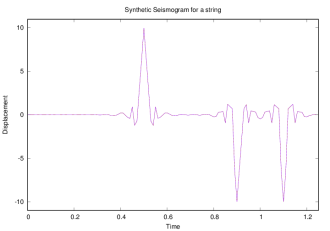
The synthetic seismogram data is saved in the file seism.dat. Now, we run the above program and plot the output.
#!/bin/bash

prog="synt_seis_strings.f" #fortran program name
exect=`echo $prog | cut -d"." -f1` #executable name

rm -f *.dat $exect #remove files

gfortran -ffree-form $prog -o $exect #compiling the fortran program
./$exect #running the executable

datascrpt='modesPlot.gp'
echo "plot [0:1.25][-8:8] 'seism.dat' using 1:2 w lines " >$datascrpt

#######GNUPLOT##################
gnuplot << EOF
fignm='synth_seis.ps'
figtitle='Synthetic Seismogram for a string'
datafile=system("echo $datascrpt")

xlb="Time"
ylb="Displacement"
set terminal postscript color solid #terminal type
set title figtitle #figure title
set xlabel xlb #xlabel
set ylabel ylb #ylabel
set output fignm #output fig name
unset key
load datafile
EOF

In the above figure, we can see three peaks. First peak at 0.5s is the direct arrival from the source to the receiver. The distance between the source and receiver is 0.5. So the time taken from the source to the receiver is 0.5/1=0.5 sec.
The other two inverted peaks are the reflected arrivals. It is the time taken by the wave from the source to reach the end and reflected back to reach the receiver. The first reflected phase we observe is at 0.9s. It it due to the reflection from the left boundary. This can be calculated ((0.2-0)+0.7)/1=0.9 sec. Similarly, the other arrival (reflected phase from the right boundary) could also be calculated.
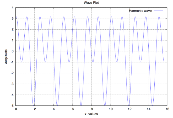
We have used the exponential source term (F(wn)=exp[-(wn*tau)^2/4] ) which depends on the value of eigenfrequencies and tau. We have modeled its dependency.

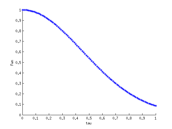
In the second figure, we have considered the value of wn=3.14.
Here, also we have considered the source term to be an exponential function. Instead, if we consider the source term to be abs(sin(x)) then we get the following synthetic seismogram.
Here, we can still see the peaks are 0.5,0.9 and 1.1 seconds but there are some wiggles are it. This is the effect of the source function. We have considered the same number of modes and other parameters.
When we consider the sinc function as the source function then the seismogram wiggles surrounding the peak decreases.
Conclusion:
In this study, we have obtained the synthetic seismogram using the normal mode summation method. We now have two ways to think of the displacement of a traveling wave, propagating waves or normal modes. These two ways can give different interesting insights about the properties of the source and the medium. The difference between the two is that in the propagating wave formulation, the travel times are measured to infer the velocity of the medium and in the normal mode formulation, eigenfrequecies are measured to infer the velocity.
The normal mode solution gives us information about the medium in which the waves propagate and the source that generates them. The physical properties of the string control its velocity (or eigenfunctions and eigenfrequencies). The displacement obtained can be used to study the source that excited them.
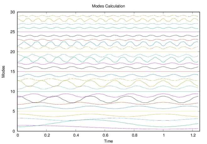
In normal mode solution, we sum all the modes to obtain the synthetic seismogram. The individual modes, though, are not physically meaningful. Each mode actually start vibrating even before the wave reaches the end of the string. But when all the modes are summed, the resulting wave propagate at the correct velocity.
In this study, we have considered a uniform string to calculate the synthetic seismogram. We could generalize this idea to obtain the modes of the non-uniform string. We can consider this case in the future posts. We can even calculate the modes for an sphere.
- Utpal Kumar (IES, Academia Sinica)