In Earth Sciences, we often deal with multidimensional data structures such as climate data, GPS data. It ‘s hard to save such data in text files as it would take a lot of memory as well as it is not fast to read, write and process it. One of the best tools to deal with such data is netCDF4. It stores the data in the HDF5 format (Hierarchical Data Format). The HDF5 is designed to store a large amount of data. NetCDF is the project hosted by Unidata Program at the University Corporation for Atmospheric Research (UCAR).
Here, we learn how to read and write netCDF4 data. We follow the workshop by Unidata. You can check out the website of Unidata.
Requirements:
Python3:
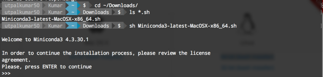
You can install Python3 via the Anaconda platform. I would recommend Miniconda over Anaconda because it is more light and installs only fundamental requirements for Python.
NetCDF4 Package:
conda install -c conda-forge netcdf4
Reading NetCDF data:
Now, we are good to go. Let’s see how we can read a netCDF data. The netCDF data has the extension of “.nc”
Importing NetCDF and Numpy ( a Python library that supports large multi-dimensional arrays or matrices):
import netCDF4
import numpy as np
Now, let us open a NetCDF Dataset object:
f = netCDF4.Dataset('../../data/rtofs_glo_3dz_f006_6hrly_reg3.nc')
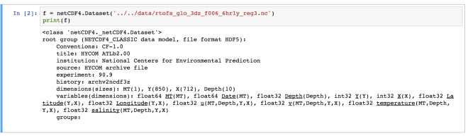
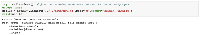
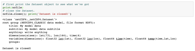
Here, we have read a NetCDF file “rtofs_glo_3dz_f006_6hrly_reg3.nc”. When we print the object “f”, then we can notice that it has a file format of HDF5. It also has other information regarding the title, institution, etc for the data. These are known as metadata.
In the end of the object file print output, we see the dimensions and variable information of the data set. This dataset has 4 dimensions: MT (with size 1), Y (size: 850), X (size: 712), Depth (size: 10). Then we have the variables. The variables are based on the defined dimensions. The variables are outputted with their data type such as float64 MT (dimension: MT).
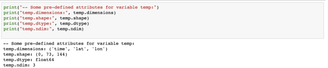
Some variables are based on only one dimension while others are based on more than one. For example, “temperature” variable relies on four dimensions – MT, Depth, Y, X in the same order.
We can access the information from this object, “f” just like we read a dictionary in Python.
print(f.variables.keys()) # get all variable names

This outputs the names of all the variables in the read netCDF file referenced by “f” object.
We can also individually access each variable:
temp = f.variables['temperature'] # temperature variable
print(temp)
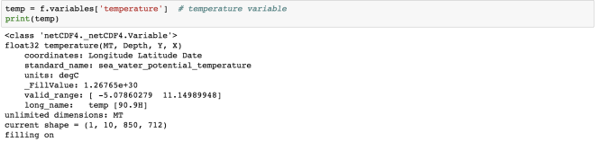
The “temperature” variable is of the type float32 and has 4 dimensions – MT, Depth, Y, X. We can also get the other information (meta-data) like the coordinates, standard name, units of the variable. Coordinate variables are the 1D variables that have the same name as dimensions. It is helpful in locating the values in time and space. The unit of temperature variable data is “degC”. The current shape gives the information about the shape of this variable. Here, it has the shape of (1, 10, 850, 712) for each dimension.
We can also check the dimension size of this variable individually:
for d in f.dimensions.items():
print(d)
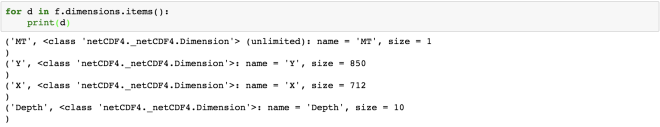
The first dimension “MT” has the size of 1, but it is of unlimited type. This means that the size of this dimension can be increased indefinitely. The size of the other dimensions is fixed.
For just finding the dimensions supporting the “temperature” variable:
temp.dimensions

temp.shape

Similarly, we can also inspect the variables associated with each dimension:
mt = f.variables['MT']
depth = f.variables['Depth']
x,y = f.variables['X'], f.variables['Y']
print(mt)
print(x)
print(y)
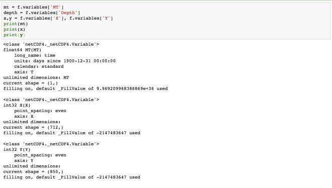
Here, we obtain the information about each of the four dimensions. The “MT” dimension, which is also a variable has a long name of “time” and units of “days since 1900-12-31 00:00:00”. The four dimensions denote the four axes, namely- MT: T, Depth: Z, X:X, Y: Y.
Now, how do we access the data from the NetCDF variable we have just read. The NetCDF variables behave similarly to NumPy arrays. NetCDF variables can also be sliced and masked.
Let us first read the data of the variable “MT”:
time = mt[:]
print(time)

Similarly, for the depth array:
dpth = depth[:]
print(depth.shape)
print(depth.dimensions)
print(dpth)

We can also apply conditionals on the slicing of the netCDF variable:
xx,yy = x[:],y[:]
print('shape of temp variable: %s' % repr(temp.shape))
tempslice = temp[0, dpth > 400, yy > yy.max()/2, xx > xx.max()/2]
print('shape of temp slice: %s' % repr(tempslice.shape))

Now, let us address one question based on the given dataset. “What is the sea surface temperature and salinity at 50N and 140W?”
Our dataset has the variables temperature and salinity. The “temperature” variable represents the sea surface temperature (see the long name). Now, we have to access the sea-surface temperature and salinity at a given geographical coordinates. We have the variables latitude and longitude as well.
The X and Y variables do not give the geographical coordinates. But we have the variables latitude and longitude as well.
lat, lon = f.variables['Latitude'], f.variables['Longitude']
print(lat)
print(lon)
print(lat[:])

Great! So we can access the latitude and longitude data. Now, we need to find the array index, say iy and ix such that Latitude[iy, ix] is close to 50 and Longitude[iy, ix] is close to -140. We can find out the index by defining a function:
# extract lat/lon values (in degrees) to numpy arrays
latvals = lat[:]; lonvals = lon[:]

# a function to find the index of the point closest pt
# (in squared distance) to give lat/lon value.
def getclosest_ij(lats,lons,latpt,lonpt):
 # find squared distance of every point on grid
 dist_sq = (lats-latpt)**2 + (lons-lonpt)**2
 # 1D index of minimum dist_sq element
 minindex_flattened = dist_sq.argmin()
 # Get 2D index for latvals and lonvals arrays from 1D index
 return np.unravel_index(minindex_flattened, lats.shape)

iy_min, ix_min = getclosest_ij(latvals, lonvals, 50., -140)
print(iy_min)
print(ix_min)

So, now we have all the information required to answer the question.
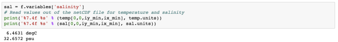
sal = f.variables['salinity']
# Read values out of the netCDF file for temperature and salinity
print('%7.4f %s' % (temp[0,0,iy_min,ix_min], temp.units))
print('%7.4f %s' % (sal[0,0,iy_min,ix_min], sal.units))
Accessing the Remote Data via openDAP:
We can access the remote data seamlessly using the netcdf4-python API. We can access via the DAP protocol and DAP servers, such as TDS.
For using this functionality, we require the additional package “siphon”:
conda install -c unidata siphon
Now, let us access one catalog data:
from siphon.catalog import get_latest_access_url
URL = get_latest_access_url('http://thredds.ucar.edu/thredds/catalog/grib/NCEP/GFS/Global_0p5deg/catalog.xml',
 'OPENDAP')
gfs = netCDF4.Dataset(URL)

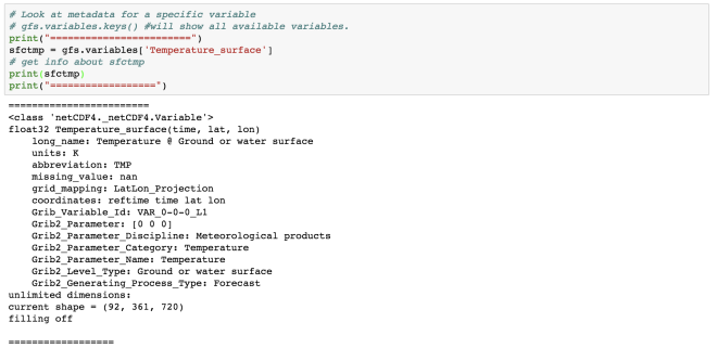
# Look at metadata for a specific variable
# gfs.variables.keys() #will show all available variables.
print("========================")
sfctmp = gfs.variables['Temperature_surface']
# get info about sfctmp
print(sfctmp)
print("==================")
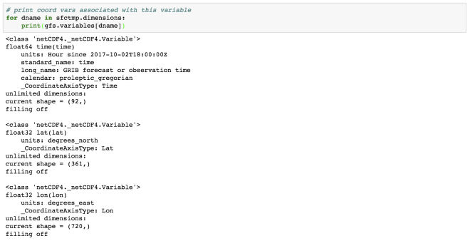
# print coord vars associated with this variable
for dname in sfctmp.dimensions:
 print(gfs.variables[dname])
Dealing with the Missing Data
soilmvar = gfs.variables['Volumetric_Soil_Moisture_Content_depth_below_surface_layer']
print(soilmvar)
print("================")
print(soilmvar.missing_value)

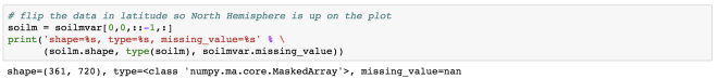
# flip the data in latitude so North Hemisphere is up on the plot
soilm = soilmvar[0,0,::-1,:]
print('shape=%s, type=%s, missing_value=%s' % \
 (soilm.shape, type(soilm), soilmvar.missing_value))
import matplotlib.pyplot as plt
%matplotlib inline
cs = plt.contourf(soilm)

Here, the soil moisture has been illustrated on the land only. The white areas on the plot are the masked values.
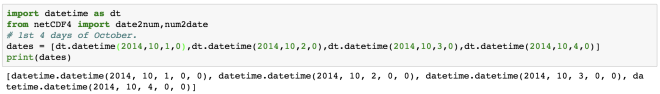
Dealing with Dates and Times
The time variables are usually measured relative to a fixed date using a certain calendar. The specified units are like “hours since YY:MM:DD hh:mm:ss”.
from netCDF4 import num2date, date2num, date2index
timedim = sfctmp.dimensions[0] # time dim name
print('name of time dimension = %s' % timedim)

Time is usually the first dimension.
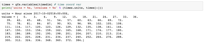
times = gfs.variables[timedim] # time coord var
print('units = %s, values = %s' % (times.units, times[:]))
dates = num2date(times[:], times.units)
print([date.strftime('%Y-%m-%d %H:%M:%S') for date in dates[:10]]) # print only first ten...

We can also get the index associated with the specified date and forecast the data for that date.
import datetime as dt
date = dt.datetime.now() + dt.timedelta(days=3)
print(date)
ntime = date2index(date,times,select='nearest')
print('index = %s, date = %s' % (ntime, dates[ntime]))
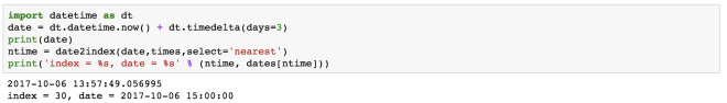
This gives the time index for a time nearest to 3 days from today, current time.
Now, we can again make use of the previously defined “getcloset_ij” function to find the index of the latitude and longitude.
lats, lons = gfs.variables['lat'][:], gfs.variables['lon'][:]
# lats, lons are 1-d. Make them 2-d using numpy.meshgrid.
lons, lats = np.meshgrid(lons,lats)
j, i = getclosest_ij(lats,lons,40,-105)
fcst_temp = sfctmp[ntime,j,i]
print('Boulder forecast valid at %s UTC = %5.1f %s' % \
 (dates[ntime],fcst_temp,sfctmp.units))

So, we have the forecast for 2017-10-06 15 hrs. The surface temperature at boulder is 304.2 K.
Simple Multi-file Aggregation
If we have many similar data, then we can aggregate them as one. For example, if we have the many netCDF files representing data for different years, then we can aggregate them as one.
Multi-File Dataset (MFDataset) uses file globbing to patch together all the files into one big Dataset.
Limitations:- It can only aggregate the data along the leftmost dimension of each variable.
- It can only aggregate the data along the leftmost dimension of each variable.
- only works with NETCDF3, or NETCDF4_CLASSIC formatted files.
- kind of slow.
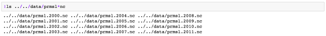
mf = netCDF4.MFDataset('../../data/prmsl*nc')
times = mf.variables['time']
dates = num2date(times[:],times.units)
print('starting date = %s' % dates[0])
print('ending date = %s'% dates[-1])
prmsl = mf.variables['prmsl']
print('times shape = %s' % times.shape)
print('prmsl dimensions = %s, prmsl shape = %s' %\
 (prmsl.dimensions, prmsl.shape))

Finally, we need to close the opened netCDF dataset.
f.close()
gfs.close()

To download the data, click here. Next, we will see how to write a netCDF data.


 Jupyter notebook can be started using the terminal. Firstly, navigate to your directory containing the data and the type “jupyter notebook” on your terminal.
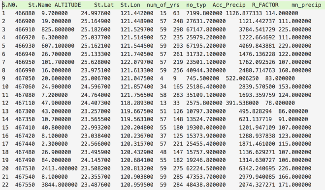
 We can see that the data has no header information, and 8 columns. The columns are namely, “year”, “latitude”, “longitude”, “Height”, “dN”, “dE”, “dU”.
 Our data is now loaded, and if we want to extract any section of the data, we can easily do that.
 Here, we have used the column names to extract the two columns only. We can also use the index values.
 When we use “.loc” method to extract the section of the data, then we need to use the column name whereas when we use the “.iloc” method then we use the index values. Here,
  We can see the “Year” column as the index of the data frame now. Plotting using Pandas is extremely easy.
 We can also customize the plot easily.
 If we want to save the figure, then we can use the command:
 This saves the figure as the pdf file named “0498Data.pdf”. The format can be set to any type “.png”, “.jpg”, ‘.eps”, etc. We set the resolution to be 300 dpi. This can be varied depending on our need. Lastly, “bbox_inches =‘tight’” crops our figure to remove all the unnecessary space.
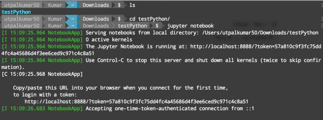
 It will open “Jupyter” in your favorite browser.