Time Series Analysis: Filtering or Smoothing the Data

In this post, we will see how we can use Python to low pass filter the 10 year long daily fluctuations of GPS time series. We need to use the “Scipy” package of Python.

The only important thing to keep in mind is the understanding of Nyquist frequency. The Nyquist or folding frequency half of the sampling rate of the discrete signal. To understand the concept of Nyquist frequency and aliasing, the reader is advised to visit this post. For filtering the time-series, we use the fraction of Nyquist frequency (cut-off frequency).

Following is the code and line by line explanation for performing the filtering in few steps:

import numpy as np #importing numpy module for efficiently executing numerical operations
import matplotlib.pyplot as plt #importing the pyplot from the matplotlib library
from scipy import signal

from matplotlib import rcParams
rcParams['figure.figsize'] = (10.0, 6.0) #predefine the size of the figure window
rcParams.update({'font.size': 14}) # setting the default fontsize for the figure
rcParams['axes.labelweight'] = 'bold' #Bold font style for axes labels
from matplotlib import style
style.use('ggplot') #I personally like to use "ggplot" style of graph for my work but it depends on the user's preference whether they wanna use it.

# - - - # We load the data in the mat format but this code will work for any sort of time series.# - - - #
dN=np.array(data['dN'])
dE=np.array(data['dE'])
dU=np.array(data['dU'])
slat=np.array(data['slat'])[0]
slon=np.array(data['slon'])[0]
tdata=np.array(data['tdata'])[0]
stn_name=np.array(stn_info['stn_name'])[0]
stns=[stn_name[i][0] for i in range(len(stn_name))]

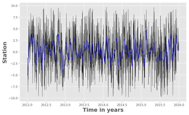
# Visualizing the original and the Filtered Time Series
fig = plt.figure()
ax = fig.add_subplot(1, 1, 1)
indx=np.where( (tdata > 2012) & (tdata < 2016) )
ax.plot(tdata[indx],dU[indx,0][0],'k-',lw=0.5)
## Filtering of the time series
fs=1/24/3600 #1 day in Hz (sampling frequency)

nyquist = fs / 2 # 0.5 times the sampling frequency
cutoff=0.1 # fraction of nyquist frequency, here  it is 5 days
print('cutoff= ',1/cutoff*nyquist*24*3600,' days') #cutoff=  4.999999999999999  days
b, a = signal.butter(5, cutoff, btype='lowpass') #low pass filter


dUfilt = signal.filtfilt(b, a, dU[:,0])
dUfilt=np.array(dUfilt)
dUfilt=dUfilt.transpose()

ax.plot(tdata[indx],dUfilt[indx],'b',linewidth=1)

ax.set_xlabel('Time in years',fontsize=18)
ax.set_ylabel('Stations',fontsize=18)
# ax.set_title('Vertical Component CGPS Data')
plt.savefig('test.png',dpi=150,bbox_inches='tight')